
One of the most important tools in statistics is the normal distribution. It aids in determining specific data features and also serves as a foundation for employing other statistical techniques for decision-making. As a result, in this article, we look at the Normal distribution and its application in real life.
In probability, the normal distribution is the most important continuous distribution in statistics because it’s common in natural phenomena. It is also known as the Gaussian distribution and is always symmetric about the mean. There are also various probability distributions such as Bernoulli, Binomial , Negative Binomial, Geometric, Hypergeometric, Poisson, Logarithmic series, Power series, Gamma, Beta, Uniform, Exponential distribution etc. But from all this normal distribution is the best measure.
| Normal curve( Bell shaped) |

What is Normal Distribution?
A normal distribution is a bell-shaped curve with a single peak for a continuous random variable. A useful continuous probability distribution is the normal distribution. The normal curve is a theoretical mathematical curve. For normal distribution, a normal curve is employed. A normal curve should be turned into a standard normal curve for practical purposes, and a given variable should be translated into a standard normal variate.
Normal distribution has two parameter μ, σ^2.
μ=population mean and
σ^2=population variance
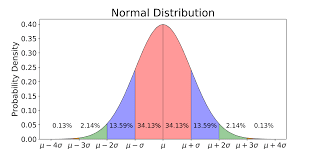
The normal curve is always in bell shape, and the mean, median, and mode is always equal. That means, mean = median = mode.
| Bell curve |
History of the Normal Distribution
In 1733, De Moivre found the normal distribution as the limiting case of the Binomial model. It has been attributed to Gauss, who first mentioned it in 1809, due to a historical error. Various attempts were made in the 18th and 19th centuries to establish the normal model as the underlying law governing all continuous random variables—hence the name Normal. Because of the incorrect premises, their initiatives failed. Nonetheless, in statistical analysis, the normal model has become the most important probability model. Gaussian distribution is another name for it.
The PDF, CDF, CF, and MGF of the normal distribution
The probability density function (PDF) is,
![\[ f(x;\mu ,\sigma )=\frac{1}{\sigma \sqrt{2\pi }}e^{-\frac{1}{2}(\frac{x-\mu }{\sigma })^{2}}; where \mu =mean,\sigma =std. \]](https://www.statisticalaid.com/wp-content/ql-cache/quicklatex.com-778df2393066c03fca7faad84cc98266_l3.png "Rendered by QuickLaTeX.com")
The Cumulative distribution function (c.d.f) is,
![\[ F(x)=\int_{0}^{\infty }f(x)dx \]](https://www.statisticalaid.com/wp-content/ql-cache/quicklatex.com-8c211d03b77cd2b2fe59c9f3995067b7_l3.png "Rendered by QuickLaTeX.com")
| CDF (cumulative density function) | |
| Mean, Median, Mode | μ |
| Variance | |
| Skewness, Kurtosis | 0 |
| MGF (moment generating function) | |
| CF |


Why is the normal distribution so common in natural phenomena?
There exist numerous natural events whose distribution follows a normal curve. Human characteristics such as weight, height, strength, body temperature, or intelligence are among those. This explanation stems from the fact that numerous independent elements (factors) impact a characteristic such as height, where these factors may work in favor or against height with a 50% chance. For example, factors such as dietary habits, genes, and lifestyle may have a positive or negative contribution to human height. Figure 1 shows a normal distribution for a height of adults in a homogeneous race.

Figure: Height of Adults in a homogeneous race and the effect of independent factors on it.
In the above Figure, the mean population height is 5’7’’. For an individual human being, each contributing factor shifts the mean population height toward left or right of 5’7’’ with a probability of 0.5. The difference between a number of factors that contribute in favor or against taller height results in the final height of a person. Assuming independence and equal importance among these factors, the probability of a person’s height being in a particular range is found by a binomial distribution.
Properties of the Normal Distribution
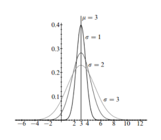
For a specific μ = 3 and a σ ranging from 1 to 3, the probability density function (P.D.F.) is as shown –
The properties are as follows –
- The distribution is symmetric about the point x = μ and has a characteristic bell-shaped curve with respect to it. Therefore, its skewness is equal to zero, i.e., the curve is neither inclined to the right (negatively skewed) nor to the left (positively skewed).
- The mean, median, and mode of a normal distribution all coincide with each other and are equal to μ.
- The Standard Deviation for this distribution is equal to σ.
Mean Deviation: σ√2.
First Quartile: μ – 0.675σ and the Third Quartile: μ + 0.675σ.
Thus, Quartile Deviation: 0.675.
Application of Normal Distribution in Business
- The so-called central limit theorem states that the normal distribution possesses a striking quality.
- Even though a variable is not normally distributed, a simple transformation of the variable can occasionally bring it into normal form.
- Many sample distributions, such as Student’s t, Student’s F, and others, tend to be normal.
- The assumption behind sampling theory and significance tests is that samples were selected from a normal population with a mean and a variance.
- The normal distribution has a lot of uses in statistical quality control.
- The normal distribution serves as a good approximation for many discrete distributions as n grows larger (such as Binomial, Poisson, etc.).
- The normal distribution has a number of mathematical properties that make it widely used and relatively simple to adjust.
The Binomial, Poisson, and Normal Distributions and Their Relationships
The Binomial, Poisson, and Normal distributions are all inextricably linked. The following are the relationships:
The Poisson and normal distributions have a connection. When n is big and the probability p of an event occurring is near to zero, the binomial distribution tends to become a Poisson distribution with np remaining a finite constant.
The binomial and normal distributions have a similar relationship. Under the following circumstances, the normal distribution is a limiting form of the binomial distribution:
- n, the number of trials is very large, i.e., n → ∞; and
- Neither p nor q is very small.
Practical Applications of the Standard Normal Model
The standard normal distribution could help you figure out which subject you are getting good grades in and which subjects you have to exert more effort in due to low scoring percentages. Once you get a score in one subject that is higher than your score in another subject, you might think that you are better in the subject where you got the higher score. This is not always true. You can only say that you are better in a particular subject if you get a score with a certain number of standard deviations above the mean. The standard deviation tells you how tightly your data is clustered around the mean; It allows you to compare different distributions that have different types of data, including different means.
For example, if you get a score of 90 in Math and 95 in English, you might think that you are better in English than in Math. However, in Math, your score is 2 standard deviations above the mean. In English, it’s only one standard deviation above the mean. It tells you that in Math, your score is far higher than most of the students (your score falls into the tail). Based on this data, you actually performed better in Math than in English!
What is the difference between normal and lognormal distributions?
| Feature | Normal Distribution | Lognormal Distribution |
|---|---|---|
| Shape | Symmetrical, bell-shaped | Skewed right (long tail on the right) |
| Value Range | Can be positive or negative | Always positive (no negative values) |
| Mean vs Median vs Mode | Mean = Median = Mode | Mean > Median > Mode |
| Common Uses | Heights, IQ scores, test results | Income, stock prices, time to failure |
| Data Behavior | Additive (linear changes) | Multiplicative (growth or decay over time) |
| Log Transformation | Log of data is not normally distributed | Log of data is normally distributed |
| Outliers | Less extreme outliers | More likely to have extreme high values |
What is lognormal distribution used for?
Here are 7 key points explaining what the lognormal distribution is used for:
- Stock Prices – Used in finance to model asset prices, since prices can’t go negative and often grow multiplicatively.
- Income & Wealth – Common in economics to model income distribution, which is usually right-skewed with a few very high earners.
- Failure Times – In engineering, used to model the lifetime of products or systems where failure happens over time.
- Biological Growth – Models things like tumor size or organism growth, which multiply over time.
- Environmental Data – Used for things like rainfall, pollution levels, and other naturally skewed measurements.
- Project Timing – Helps estimate completion times when tasks are uncertain and can vary widely.
- Right-Skewed Data – In general, used whenever data is strictly positive and has a long tail of larger values.
Conclusion
In the natural and behavioral sciences, the normal distribution is a useful model for quantitative phenomena. A normal distribution has been found to roughly follow a number of psychological test scores and physical phenomena such as photon counts. While the underlying reasons for these events are frequently unknown, the usage of the normal distribution in cases where several minor effects are compounded together to produce a score or variable that can be observed is logically appropriate. The normal distribution also appears in many fields of statistics: for example, even if the distribution of the population from which the sample was taken is not normal, the sampling distribution of the mean is approximately normal. Furthermore, among all distributions with known mean and variance, the normal distribution maximizes information entropy, making it the natural choice as the underlying distribution for data summarized in terms of sample mean and variance. Data Science Blog
Variable transformation, Recoding variables in spss
Univariate Analysis (data analysis using spss part-9)
Bivariate analysis| How to analyze data using spss (part-10)
Normality check| how to analyze data using spss (part-11)