
The binomial distribution is a cornerstone of probability and statistics, frequently popping up in fields ranging from scientific research to marketing analytics. While the name might sound intimidating, understanding its core principles unlocks a powerful tool for predicting and analyzing events with binary outcomes – think coin flips, survey responses, or website conversions.
Binomial distribution was discovered by James Bernoulli (1654-1705) in the year 1700 and was first published posthumously in 1713, eight years after his death. Let a random experiment be performed repeatedly, each repetition being called a trial and let the occurrence of an event in a trial be called a success and its non-occurrence a failure. Consider a set of n (finite) independent Bernoulli trials in which the probability ‘p’ of success in any trial is constant for each trial, then q=1-p, is the probability of failure in any trial.

What is the Binomial Distribution?
Binomial distribution is a special case of Bernoulli distribution where the number of trial is up to n times instead of two times ( probability of success “p” and probability of failure “q”).
Let X be a discrete random variable, X is said to have binomial distribution if the density of X is defined as,
![\[ f(X=r;n,p)=\left ( _{r}^{n}\textrm{} \right )p^{r}q^{1-r}; where, (_{r}^{n}\textrm{})=\frac{n!}{r!(n-r)!} for.. r=0,1,2,...,n \]](https://www.statisticalaid.com/wp-content/ql-cache/quicklatex.com-1723f2bcd035553594e73f6736aa24ca_l3.png "Rendered by QuickLaTeX.com")
Here , n = total number of observation
r = number of trial
p = probability of success
q = probability of failure
So the probability distribution of X is called the binomial distribution. This is a discrete probability distribution.
The two independent constant n and p in the distribution are known as the parameter of the distribution. ‘n’ is also sometimes, known as the degree of the binomial distribution. Binomial distribution is a discrete distribution as X can take only the integral value, 0,1,2,…,n. Any random variable which follow binomial distribution is known as binomial variate.
Properties of Binomial Distribution
- Fixed number of trials, n, which means that the experiment is repeated a specific number of times.
- The n trials are independent, which means that what happens on one trial does not influence the outcomes of other trials.
- There are only two outcomes, which are called a success and a failure.
- The probability of a success doesn’t change from trial to trial, where p = probability of success and q = probability of failure, q = 1 – p .
Mean and Variance of Binomial distribution
Understanding the central tendency and spread of a binomial distribution is crucial for interpretation. The mean (average) and variance provide these key insights.
- Mean (μ): The average number of successes expected in n trials. It is calculated as: μ = np; that means, Mean(X)= µ = E(X) = np.
- Variance (σ²): A measure of the spread or dispersion of the distribution. It is calculated as: σ² = np(1 – p); that means Variance(X)=σ2 = V (X) = np(1 − p) .
- Standard Deviation (σ): The square root of the variance, providing a more interpretable measure of spread in the same units as the original data.σ = √(np(1 – p))
For example, in the coin flip scenario with 5 flips and a probability of heads of 0.5:
- μ = 5 * 0.5 = 2.5 (We expect an average of 2.5 heads)
- σ² = 5 * 0.5 * 0.5 = 1.25
- σ = √1.25 ≈ 1.12
PMF, CDF and Inverse CDF
Manually calculating binomial probabilities can be time-consuming, especially for larger values of n. Statistical software packages like R, Python (with libraries like SciPy), SPSS, and even spreadsheet programs like Excel offer built-in functions to streamline these calculations. These functions typically include:
- Probability Mass Function (PMF): Calculates the probability of exactly k successes (P(X = k)).
- Cumulative Distribution Function (CDF): Calculates the probability of k or fewer successes (P(X ≤ k)).
- Inverse CDF (Quantile Function): Finds the value of k corresponding to a given cumulative probability.
Learning to use these functions within your chosen software package will significantly enhance your ability to apply the binomial distribution in practice.
Applications of the Binomial Distribution: Real-World Examples
The binomial distribution finds applications in diverse fields:
- Quality Control: Assessing the probability of defective items in a production batch. Manufacturers use this to determine if a batch meets quality standards.
- Marketing: Predicting the success rate of a marketing campaign based on historical conversion data. Helps in budgeting and campaign optimization.
- Medicine: Determining the effectiveness of a new drug or treatment in clinical trials. Evaluates if the treatment significantly improves patient outcomes.
- Genetics: Analyzing the probability of inheriting a specific trait from parents.
- Polling and Surveys: Estimating the proportion of a population that holds a particular opinion. Provides insights into public sentiment and political leanings.
- Finance: Modeling the probability of a stock price going up or down over a certain period.
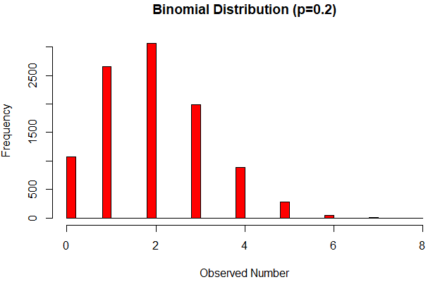
Shape of Binomial Distribution
The shape or pattern of binomial distribution depends on the values of p and n. If p=q=0.5, the distribution will be symmetrical regardless of the values of n. If p≠q, the distribution will be asymmetrical. Given a particular n, the more the difference between p and q , the greater the skewness of the distribution will be. When p<q , the distribution will be positively skewed and when p>q then the distribution will be negatively skewed. However as the value of n increases, the distribution will become less and less skewed. When n becomes infinitely large, the distribution will approach symmetry irrespective of the difference between p and q.
The effects of increases in n on the shape of the binomial distribution are shown in the below figure. The first set of figures is drawn on the assumption that p=q. The distribution is always symmetrical. As the value of n increases, the bars become narrower and more numerous. As n approaches infinity, the bars become vertical lines with no space in between, and the distribution becomes bell-shaped smooth curve.
And the second set of figures in drawn on the assumption that the probability of a success on a single trial is 0.1. It shows that as n become larger and larger, the skewness of the distribution disappears and in the long run the distribution becomes continuous. Thus it is apparent that as the value of n increases, the binomial distribution becomes a continuous and symmetrical distribution whether or not p and q are equal.
Real Life examples of Binomial Distribution
There are many, many excellent examples —
- We can see from baby that born, there are two options between boy or girl and binomial distribution was used to predict that baby is girl or boy.
- In a manufacturing context, the number of faulty items in a batch of products might follow a binomial distribution, if the probability of failures is constant. In practice, this probably isn’t true, because of the chance that an equipment failure generates clusters of failures. I vaguely remember doing a project about 45 years ago on failures of welds, where the number of failures in a particular product was in practice very close to the expected binomial distribution, with something like n=40 and p=0.01 (roughly 67% 0 fails, 27% 1 fail, 6% more than 1).
- A chart of height for adult males in any given country, or adult females in any given country, will follow a binomial distribution (the famous “bell curve”) beautifully, in which the curve is very high around the average and then tapers off in either direction. Exactly as the binomial distribution predicts, there will be a few “outliers”… people exceptionally above or below average, but their numbers will be extremely small, approaching zero as you get farther away from the average.
When Not to Use the Binomial Distribution
While powerful, the binomial distribution isn’t a one-size-fits-all solution. Here are some situations where it’s inappropriate:
- Trials are not independent: If the outcome of one trial influences the outcome of another (e.g., sampling without replacement from a small population).
- More than two outcomes: If each trial can result in more than two possibilities (e.g., the type of car someone drives). For these scenarios, other distributions like the multinomial distribution are more appropriate.
- Probability of success changes: If the probability of success varies from trial to trial (e.g., an employee learning a task, where their success rate increases over time).
- Infinite or undefined number of trials: The binomial distribution requires a fixed, known number of trials.
Binomial distribution Calculator

Example 1: Coin Flips
You flip a fair coin 5 times. What is the probability of getting exactly 3 heads?
- n = 5 (number of trials)
- k = 3 (number of successes – heads)
- p = 0.5 (probability of success on a single trial – getting heads)
- (1 – p) = 0.5 (probability of failure on a single trial – getting tails)
First, calculate the binomial coefficient:
(5 C 3) = 5! / (3! * 2!) = (5 * 4 * 3 * 2 * 1) / ((3 * 2 * 1) * (2 * 1)) = 10
Now, plug the values into the binomial formula:
P(X = 3) = (10) * (0.5)^3 * (0.5)^(5 – 3) = 10 * 0.125 * 0.25 = 0.3125
Therefore, the probability of getting exactly 3 heads in 5 coin flips is 0.3125, or 31.25%.
Example 2: Website Conversions
A website has a conversion rate of 2% (meaning 2% of visitors make a purchase). If 200 people visit the website in a day, what is the probability that exactly 5 of them will make a purchase?
- n = 200 (number of trials – website visitors)
- k = 5 (number of successes – conversions)
- p = 0.02 (probability of success on a single trial – conversion)
- (1 – p) = 0.98 (probability of failure on a single trial – no conversion)
Calculating (200 C 5) by hand can be tedious. Statistical software or calculators with built-in functions can help. Using a calculator, we find:
(200 C 5) ≈ 2.535 * 10^9 (2.535 billion)
Now, plug the values into the binomial formula:
P(X = 5) ≈ (2.535 * 10^9) * (0.02)^5 * (0.98)^(200 – 5) ≈ 0.036
Therefore, the probability of exactly 5 people making a purchase out of 200 website visitors, given a 2% conversion rate, is approximately 0.036, or 3.6%.
Conclusion
The binomial distribution is a fundamental tool for understanding and analyzing events with binary outcomes. By grasping its core principles, understanding the formula, and exploring its diverse applications, you can leverage its power to make informed decisions in various fields. Whether you’re analyzing website conversion rates, evaluating the effectiveness of a new drug, or simply predicting the outcome of a coin flip, the binomial distribution provides a valuable framework for interpreting data and making data-driven predictions. So, dive in, practice with examples, and unlock the potential of this powerful statistical tool!