Probability Density Function (PDF)

Probability plays a crucial role in statistics, data science, and various fields where uncertainty and randomness are involved. One of the fundamental concepts within probability theory is the Probability Density Function (PDF). This blog post aims to provide an in-depth understanding of the PDF, its significance, how it works, and practical applications. By the end, you will have a clear grasp of this core statistical tool, along with a conclusion and a helpful Q&A section.

What is a Probability Density Function?

A Probability Density Function (PDF) is a function that describes the likelihood of a continuous random variable taking on a specific value. Unlike discrete random variables, which have Probability Mass Functions (PMF) assigning probabilities to distinct points, continuous variables can take any value in an interval, so we use PDFs to describe the distribution of probabilities over a range of values.

Key Characteristics of a PDF:

Continuous Variable: PDFs apply to continuous random variables such as height, weight, or temperature.
Non-negative Values: The PDF value for any point is always greater than or equal to zero, f(x)≥0.
Area Under Curve = 1: The total area under the curve of a PDF over the entire range of possible values equals 1, representing the certainty that the variable falls somewhere in the range.
Probability from Area: The probability that the variable falls within a specific interval [a,b] is given by the area under the PDF curve between a and b.

Mathematically, if X is a continuous random variable with PDF f(x), the probability that X falls between two points aaa and bbb is:

$P(a \leq X \leq b) = \int_{a}^{b} f(x)\, dx$

The probability at a single point x is technically zero because the area under a curve at a specific point has no width, but the PDF value at x, f(x), itself provides useful information about the density of probability around x.

Understanding PDFs Through Examples

Example 1: Uniform Distribution

Consider a continuous random variable X uniformly distributed between 0 and 1. The PDF is:

$f(x) = \begin{cases} 1 & \text{if } 0 \leq x \leq 1 \\ 0 & \text{otherwise} \end{cases}$

This means the probability density is constant across the interval, and the total area under the curve is 1. The probability of X falling between 0.3 and 0.6 is the area of the rectangle:

$P(0.3 \leq X \leq 0.6) = 0.6 - 0.3 = 0.3$

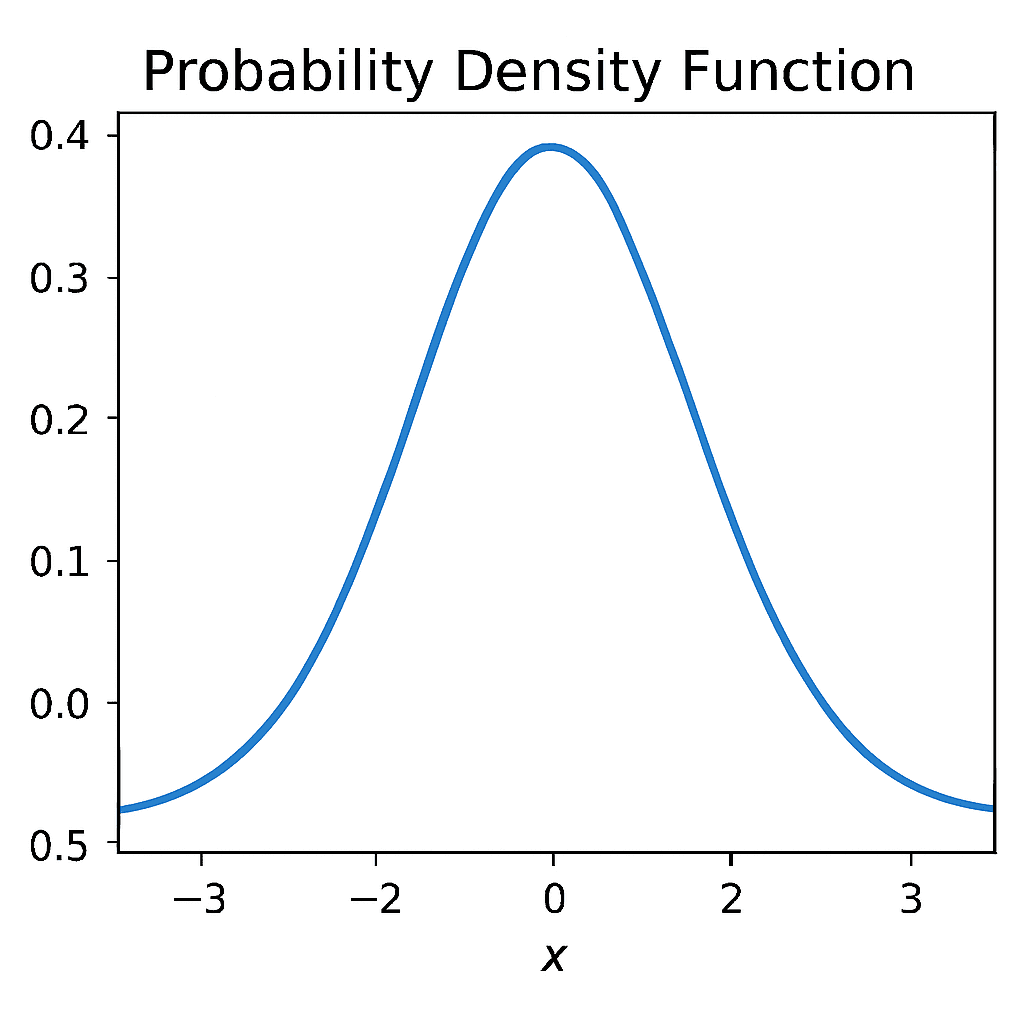
Example 2: Normal Distribution

The most famous PDF is that of the normal (Gaussian) distribution:

$f(x) = \frac{1}{\sigma \sqrt{2\pi}} \; e^{-\frac{(x-\mu)^2}{2\sigma^2}}$

where μ is the mean and σ is the standard deviation.

The normal distribution has a bell shape and is symmetric about the mean. Its PDF describes values that cluster around μ\muμ with probabilities tapering off as you move further away.

Properties of Probability Density Functions

Normalization: Ensuring the total area under the curve equals 1.
Non-negativity: f(x)≥0 for all x.
Cumulative Distribution Function (CDF): This function F(x) represents the cumulative probability up to x:

$F(x) = P(X \leq x) = \int_{-\infty}^{x} f(t)\, dt$

The CDF is a non-decreasing function that moves from 0 to 1 as x moves from negative infinity to positive infinity.

Expectation and Variance: The expected value (mean) of a continuous random variable is:

$E(X) = \int_{-\infty}^{\infty} x f(x)\, dx$

The variance measures spread:

$\mathrm{Var}(X) = \int_{-\infty}^{\infty} (x - E(X))^2 f(x)\, dx$

Applications of Probability Density Functions

1. Data Science and Machine Learning

In data science and machine learning, PDFs are essential for modeling and understanding how data is distributed. Algorithms like Gaussian Naive Bayes use normal distributions to estimate the likelihood of features given class labels. PDFs are used in density estimation, anomaly detection, and probabilistic deep learning models like variational autoencoders (VAEs).

2. Physics

In physics, PDFs describe the probabilistic nature of phenomena at both microscopic and macroscopic scales. In quantum mechanics, a particle’s wave function squared gives the probability density of its likely position.

3. Finance

In finance, PDFs provide a mathematical framework for quantifying uncertainty and risk. They model asset returns and price derivatives, as in Black–Scholes, assuming log-normal stock prices. Beyond options, PDFs support risk assessment, portfolio optimization, and Value-at-Risk (VaR) calculations.

4. Engineering

In engineering, PDFs are widely used to analyze noise, uncertainty, and system reliability. And also, PDFs model noise in signal processing, helping design filters and error-correction systems. They also describe system reliability, aiding maintenance planning and predicting component lifetimes under uncertainty.

5. Healthcare and Medicine

In healthcare and medicine, PDFs help model uncertainties in patient outcomes, disease progression, and treatment efficacy. Survival analysis often uses exponential or Weibull distributions to estimate patient survival probabilities. PDFs are also applied in epidemiology and medical imaging to study variability, aiding clinical decisions and risk management.

Visualizing Probability Density Functions (PDFs)

Visualizing a Probability Density Function provides an intuitive way to understand how probabilities are distributed across different values of a random variable. A graph of the PDF against its variable illustrates where the variable is more likely or less likely to fall. The total area under the curve equals 1, and the area between two points on the horizontal axis represents the probability of the variable lying within that interval.

One way to think about a PDF is as a probability landscape: tall peaks highlight values that occur more frequently, while flat or low regions correspond to less likely outcomes. For instance, the bell-shaped curve of the normal distribution emphasizes that most observations cluster around the mean, with probabilities tapering off symmetrically toward the extremes. By visualizing PDFs, researchers and analysts can quickly interpret patterns, compare distributions, and identify unusual or extreme values.

Practical Computation of Probabilities

While the concept of a PDF is mathematically elegant, actually computing probabilities often requires more than just writing down a formula. In practice, we determine the probability of a variable falling within a range by evaluating the integral of the PDF across that range. For simple distributions—such as the uniform distribution, where probabilities spread evenly, or the exponential distribution, which decays predictably—we can calculate these probabilities directly using closed-form expressions.

However, for more complex distributions like the normal distribution or the gamma distribution, the integrals do not always yield neat solutions. Instead, statisticians rely on numerical methods, software packages, or precomputed resources such as z-tables and chi-square tables. Modern tools like R, Python, and MATLAB make these computations efficient and accurate, enabling researchers to handle real-world data without being limited by the complexity of the underlying math.

Conclusion

The Probability Density Function is one of the cornerstones of probability and statistics, serving as a bridge between theoretical mathematics and practical applications. By showing how probabilities are distributed over a continuum of values, PDFs allow us to model uncertainty, estimate risks, and make informed predictions. From finance and engineering to medicine and artificial intelligence, the concept of the PDF underpins critical decisions and scientific discoveries.

Understanding PDFs strengthens statistical reasoning and provides a foundation for advanced topics like cumulative distribution functions and hypothesis testing. Mastering PDFs is crucial for learning Bayesian inference and other probabilistic methods applied in real-world data analysis. Grasping PDFs helps anyone interpret uncertainty and the mathematical structures that model and explain real-world phenomena effectively. Data Science Blog

Q&A Section

Q1: What is the difference between a Probability Density Function and a Probability Mass Function?

A1: A Probability Mass Function (PMF) applies to discrete random variables and assigns probabilities to exact values, while a Probability Density Function (PDF) applies to continuous random variables and describes the density of probabilities over an interval. The probability for a specific value in a PDF is zero; only intervals have positive probability.

Q2: Can PDF values be greater than 1?

A2: Yes, PDF values can be greater than 1 as long as the total area under the curve sums to 1. A PDF value is a density, not a probability by itself.

Q3: How is the cumulative distribution function (CDF) related to the PDF?

A3: The CDF is the integral (area under the curve) of the PDF from negative infinity up to a value xxx. It represents the cumulative probability that the variable is less than or equal to xxx.

Q4: Is the area under a PDF curve always equal to 1?

A4: Yes, by definition, the total area under a PDF over the entire range of the random variable is always 1, representing total certainty that the variable takes some value within that domain.

Q5: Why is the probability at a single point in a continuous distribution zero?

A5: Because the probability is represented as an area under the curve, and a single point has no width, the area (probability) at one point is zero. Probabilities are meaningful only over intervals.

By understanding these fundamentals and how to work with PDFs, you can better handle various data modeling tasks and effectively interpret continuous probability distributions.