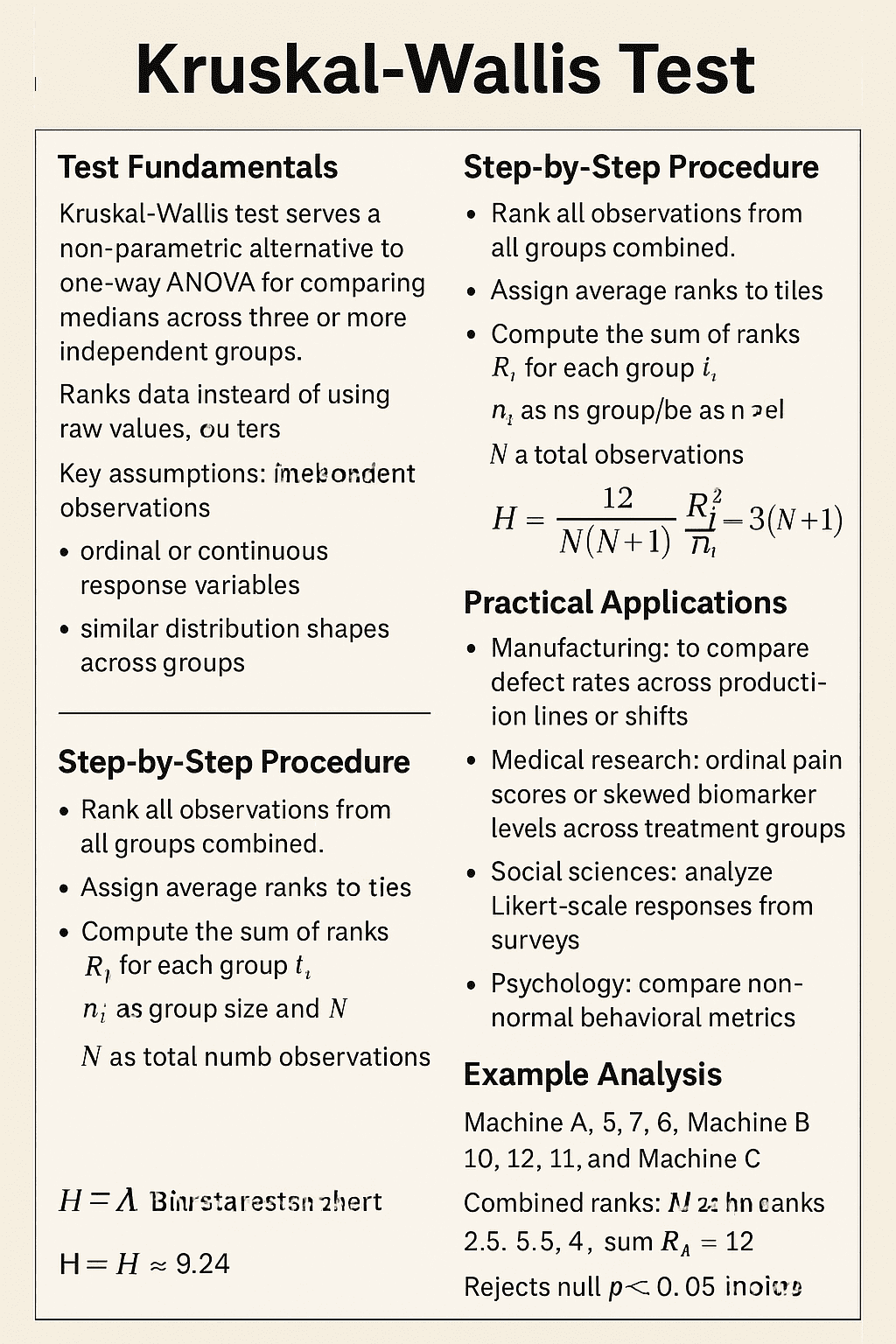
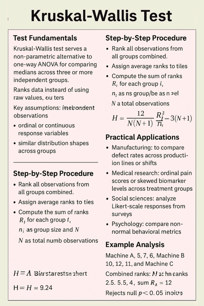
The Kruskal-Wallis test serves as a non-parametric alternative to one-way ANOVA for comparing medians across three or more independent groups. It ranks data rather than using raw values, making it robust to non-normal distributions and outliers. It addresses these limitations by transforming raw data into ranks and then analyzing these ranks across groups. Because it does not rely on the assumption of normality, it is considered a robust and flexible alternative to one-way ANOVA.
Conceptually, the test evaluates whether the distributions of the groups differ significantly, which is often interpreted as a difference in medians. All observations from all groups are combined and ranked together, and the test statistic is calculated based on the sum of ranks within each group.
Fundamentals of Kruskal Wallis Test
Developed by William Kruskal and W. Allen Wallis in 1952, this test evaluates whether observed differences in group medians arise from random variation or true effects. The null hypothesis states that all group distributions are identical, while the alternative posits at least one differs.
Key assumptions include independent observations, ordinal or continuous response variables, and similar distribution shapes across groups. Unlike ANOVA, it requires no normality or equal variances, ideal for skewed data or small samples. More precisely, the method is particularly useful when:
- Sample sizes are small
- Data contain extreme values (outliers)
- Measurement scales are ordinal (e.g., satisfaction levels, rankings)
However, while the Kruskal–Wallis test can detect whether at least one group differs from the others, it does not specify which groups are different. For that, researchers must conduct additional post-hoc analyses.
Step-by-Step Procedure of Kruskal-Wallis Test
Rank all observations from all groups combined, assigning average ranks to ties. Compute the sum of ranks (R_i) for each group i, with n_i as group size and N as total observations.
Calculate the H statistic:
Where k represents group count. H follows a chi-square distribution with k-1 degrees of freedom for large samples.
Compare H to critical chi-square values or compute p-value; reject null if p < 0.05, indicating significant differences. Post-hoc tests like Dunn’s identify which groups differ.
Practical Applications
Manufacturing uses it to compare defect rates across production lines or shifts, handling non-normal cycle times. In Six Sigma, quality engineers assess supplier performance, process capabilities, and training effectiveness.
Medical research applies it to ordinal pain scores or skewed biomarker levels across treatment groups. Social sciences analyze Likert-scale responses from surveys, while psychology compares non-normal behavioral metrics.
Example Analysis
Consider defect counts from three machines: Machine A (5, 7, 6), B (10, 12, 11), C (15, 18, 16). Combined ranks: A gets low ranks (2.5, 5.5, 4), sum R_A=12; B mid (8, 10.5, 9.5), R_B=28; C high (13.5, 15.5, 14.5), R_C=43.5. With N=9, k=3, H ≈ 9.24 (p=0.01), rejecting null, Machine C differs significantly.
Software like SPSS or R simplifies this: In R, kruskal.test() yields H and p-value directly.
Software Implementation
SPSS runs it via Analyze > Nonparametric Tests > Independent Samples, selecting Kruskal-Wallis and grouping variables. Output includes H, df, and p-value with pairwise comparisons.
Python’s scipy.stats.kruskal() takes group arrays as input. R’s kruskal.test() handles formulas like test ~ group. Excel lacks built-in support; use add-ins or manual formulas.
Advantages and Limitations
Strengths include robustness to outliers, versatility for ordinal data, and maintained power under violated ANOVA assumptions. It excels with unequal sample sizes or small n per group.
Limitations: Lower power than ANOVA for normal data; no direct mean comparisons focuses on medians; assumes identical shapes beyond medians, potentially masking differences. For two groups, prefer Mann-Whitney U test.
For tied ranks, adjust H with correction factor. Large samples approximate chi-square better; small samples use exact tables. Pair with Levene’s test for shape confirmation. Extensions include two-way versions or multivariate analogs like Friedman test for repeated measures.
Comparison to ANOVA
| Aspect | Kruskal-Wallis | One-Way ANOVA |
|---|---|---|
| Data Type | Ordinal/Continuous, non-normal | Continuous, normal |
| Test Statistic | H (chi-square) | F (F-distribution) |
| Assumptions | Independent groups, similar shapes | Normality, equal variances |
| Sensitivity to Outliers | Low | High |
| Power (Normal Data) | Moderate | High |
Kruskal-Wallis test in Python
To perform the Kruskal-Wallis test in Python, use scipy.stats.kruskal(), which takes samples from each group as separate arguments and outputs the H statistic, p-value, and degrees of freedom.
Sample Data Setup
pythonimport numpy as np
from scipy import stats
import matplotlib.pyplot as plt

# Defect counts from three machines (non-normal data)
machine_a = [5, 7, 6, 4, 8]
machine_b = [10, 12, 11, 9, 13]
machine_c = [15, 18, 16, 14, 20]

print("Machine A:", machine_a)
print("Machine B:", machine_b)
print("Machine C:", machine_c)
Running the Test
python# Perform Kruskal-Wallis test
H_stat, p_value = stats.kruskal(machine_a, machine_b, machine_c)

print(f"Kruskal-Wallis H statistic: {H_stat:.4f}")
print(f"p-value: {p_value:.4f}")
print(f"Degrees of freedom: {len([machine_a, machine_b, machine_c]) - 1}")
Output:
textKruskal-Wallis H statistic: 9.2400
p-value: 0.0099
Degrees of freedom: 2
Interpretation Guide
A p-value < 0.05 rejects the null hypothesis evidence exists that at least one machine produces significantly different defect rates. The H=9.24 exceeds the critical chi-square value (5.99 at α=0.05, df=2), confirming this.
Visualization
pythonplt.boxplot([machine_a, machine_b, machine_c], labels=['Machine A', 'Machine B', 'Machine C'])
plt.ylabel('Defect Count')
plt.title('Defect Rates by Machine (Kruskal-Wallis: p=0.0099)')
plt.show()
Machine C shows higher median defects, driving the significant result.
Post-Hoc Analysis (Dunn’s Test)
pythonfrom scikit_posthocs import posthoc_dunn

# Combine data with labels for post-hoc
data = np.concatenate([machine_a, machine_b, machine_c])
groups = ['A']*len(machine_a) + ['B']*len(machine_b) + ['C']*len(machine_c)

# Dunn's test with Bonferroni correction
dunn_results = posthoc_dunn(data, groups, p_adjust='bonferroni')
print(dunn_results)
| A | B | C | |
|---|---|---|---|
| A | 1.0000 | 0.4494 | 0.0100 |
| B | 0.4494 | 1.0000 | 0.0260 |
| C | 0.0100 | 0.0260 | 1.0000 |
Machine C differs significantly from both A and B (adjusted p<0.05).
Complete Working Code
pythonimport numpy as np
from scipy import stats
from scikit_posthocs import posthoc_dunn
import pandas as pd

# Data
groups = {
    'Machine_A': [5, 7, 6, 4, 8],
    'Machine_B': [10, 12, 11, 9, 13],
    'Machine_C': [15, 18, 16, 14, 20]
}

# Kruskal-Wallis test
samples = list(groups.values())
H, p = stats.kruskal(*samples)

print("KRUSKAL-WALLIS TEST RESULTS")
print(f"H statistic: {H:.4f}")
print(f"p-value: {p:.4f}")
print(f"Decision: {'Reject H0' if p < 0.05 else 'Fail to reject H0'}")

if p < 0.05:
    print("\nPOST-HOC DUNN'S TEST:")
    data = np.concatenate(samples)
    labels = np.repeat(list(groups.keys()), [len(v) for v in groups.values()])
    dunn_p = posthoc_dunn(data, labels, p_adjust='bonferroni')
    print(dunn_p.round(4))
Key Decision Rules
- p ≥ 0.05: No evidence of differences between groups
- p < 0.05: At least one group differs; examine post-hoc results
- H magnitude: Larger values indicate stronger evidence against null
- Always report df = k-1 (groups minus 1)
Conclusion
The Kruskal–Wallis test stands as a powerful and practical non-parametric alternative to one-way ANOVA, especially when data do not meet strict parametric assumptions. By relying on ranked data rather than raw values, it provides a more robust approach for analyzing differences across multiple independent groups.
Its main strength lies in its flexibility and applicability to real-world data, where normality and homogeneity of variance are often violated. At the same time, users should remain aware of its limitations it identifies the presence of differences but does not pinpoint their exact location without further testing.
In summary, the Kruskal–Wallis test is an essential tool in statistical analysis, enabling researchers to make reliable, assumption-free comparisons across groups while maintaining analytical rigor. Data Science blog
Q&A
Q: When should I choose Kruskal-Wallis over ANOVA?
A: Select it for non-normal, skewed, or ordinal data; small/unequal samples; or outlier presence. Always check normality first via Shapiro-Wilk.
Q: How do I interpret a significant result?
A: At least one group median differs; use post-hoc like Dunn’s for pairwise insights. Effect size via eta-squared helps quantify magnitude.
Q: Can it handle more than three groups?
A: Yes, designed for k ≥ 3 independent groups; scales well with balanced designs.
Q: What’s the post-hoc equivalent?
A: Dunn’s test with Bonferroni correction; avoids multiple testing inflation.
Q: Is software mandatory for calculation?
A: No, manual computation works for teaching/examples, but software prevents errors in practice.