PCA means Principal Component Analysis. Principal Component Analysis (PCA) is a powerful dimensionality reduction technique widely used in statistics, machine learning, and data analysis. In simpler terms, it’s a way to simplify complex data by reducing the number of variables while retaining the most important information. PCA is a multivariate technique that is used to reduce the dimension of a dataset. More precisely, PCA is concerned with explaining the variance-covariance structure through a few linear combinations of the original variables. Thus, PCA transforms the original set of variables into a smaller set of linear combinations that account for most of the variance of the original set.
Objectives of PCA
There are two main objectives of PCA. They are,
- Data reduction: Although p-components reproduce the total variability, often much of the variability can be accounted for by a small number, say k, of the PCs.
- Interpretation: Analysis of PCs often reveals relationships that were not previously suspected and thereby allows interpretations that would not ordinarily result.
PCA is also used for the following purposes:
- PCA can give the best linearly independent and different combinations of features so we can use them to describe our data differently.
- More Realistic Perspective and Less Complexity.
- Better visualization.
- Reduce size.
How PCA Works: A Step-by-Step Overview
Here’s a simplified breakdown of the PCA process:
- Data Standardization: PCA is sensitive to the scale of the variables. So, the first step is to standardize the data. This involves subtracting the mean from each variable and dividing by its standard deviation, resulting in variables with a mean of 0 and a standard deviation of 1. This ensures that all variables contribute equally to the analysis.
- Covariance Matrix Calculation: The covariance matrix describes the relationships between the variables. It tells us how much each pair of variables varies together.
- Eigenvalue Decomposition: This is where the magic happens! We decompose the covariance matrix into its eigenvectors and eigenvalues.
- Eigenvectors: These are the directions of the principal components. Each eigenvector represents a direction in the original feature space.
- Eigenvalues: These represent the amount of variance explained by each eigenvector (principal component). Larger eigenvalues correspond to more significant components.
- Selecting Principal Components: We sort the eigenvalues in descending order and choose the top k eigenvectors, where k is the desired number of principal components. The choice of k depends on the desired level of dimensionality reduction and the amount of variance you want to retain. A common approach is to choose k such that the selected components explain a certain percentage (e.g., 95%) of the total variance.
- Feature Transformation: Finally, we transform the original data by projecting it onto the selected principal components. This creates a new dataset with k features, which are the principal components.
R code of Principal Component Analysis (PCA)
##First, load the package:

library("factoextra")

##Input/Insert/Load your data set:
##For example we use a data set data(decathlon2)

data(decathlon2)
decathlon2.active <- decathlon2[1:23, 1:10]
decathlon2.active

##Performing PCA:

res.pca <- prcomp(decathlon2.active, scale = TRUE)
fviz_eig(res.pca)
fviz_pca_ind(res.pca,
col.ind = "cos2",
gradient.cols = c("#00AFBB", "#E7B800", "#FC4E07"),
repel = TRUE)
viz_pca_var(res.pca,
col.var = "contrib",
gradient.cols = c("#00AFBB", "#E7B800", "#FC4E07"),
repel = TRUE)
fviz_pca_biplot(res.pca, repel = TRUE,
col.var = "#2E9FDF",
col.ind = "#696969")

###Access to the PCA results:

eig.val <- get_eigenvalue(res.pca)
eig.val
Results of Principal Component Analysis
The Scree plot of the dataset is as follows,
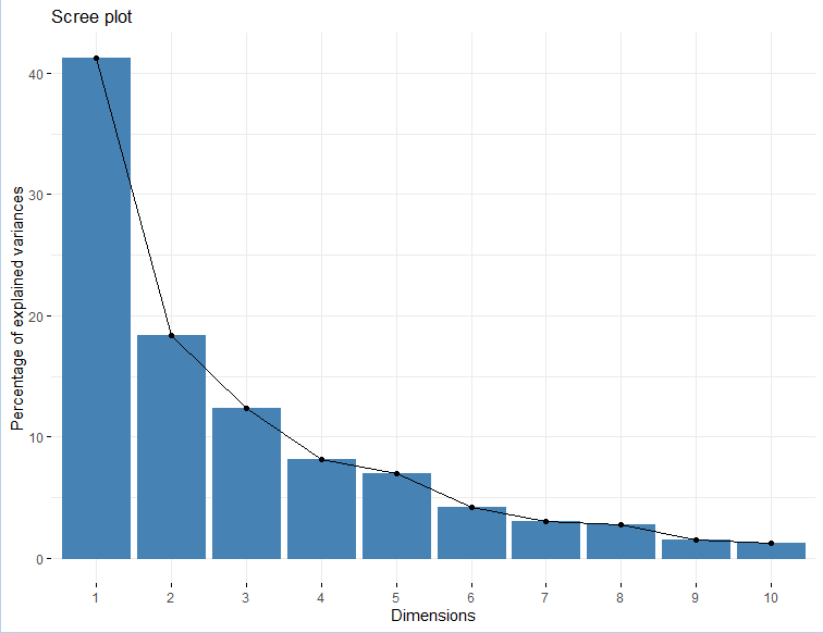
Eigenvalues and Factors
##Eigen values
 eigenvalue variance.percent cumulative.variance.percent
Dim.1   4.1242133        41.242133                    41.24213
Dim.2   1.8385309        18.385309                    59.62744
Dim.3   1.2391403        12.391403                    72.01885
Dim.4   0.8194402         8.194402                    80.21325
Dim.5   0.7015528         7.015528                    87.22878
Dim.6   0.4228828         4.228828                    91.45760
Dim.7   0.3025817         3.025817                    94.48342
Dim.8   0.2744700         2.744700                    97.22812
Dim.9   0.1552169         1.552169                    98.78029
Dim.10  0.1219710         1.219710                   100.00000


res.ind <- get_pca_ind(res.pca)
res.ind$coord
res.ind$contrib
res.ind$cos2
###
 Dim.1      Dim.2       Dim.3       Dim.4         Dim.5       Dim.6
SEBRLE       0.1912074 -1.5541282 -0.62836882  0.08205241  1.1426139415 -0.46389755
CLAY         0.7901217 -2.4204156  1.35688701  1.26984296 -0.8068483724  1.30420016
BERNARD     -1.3292592 -1.6118687 -0.19614996 -1.92092203  0.0823428202 -0.40062867
YURKOV      -0.8694134  0.4328779 -2.47398223  0.69723814  0.3988584116  0.10286344
ZSIVOCZKY   -0.1057450  2.0233632  1.30493117 -0.09929630 -0.1970241089  0.89554111
McMULLEN     0.1185550  0.9916237  0.84355824  1.31215266  1.5858708644  0.18657283
MARTINEAU   -2.3923532  1.2849234 -0.89816842  0.37309771 -2.2433515889 -0.45666350
HERNU       -1.8910497 -1.1784614 -0.15641037  0.89130068 -0.1267412520  0.43623496
BARRAS      -1.7744575  0.4125321  0.65817750  0.22872866 -0.2338366980  0.09026010
NOOL        -2.7770058  1.5726757  0.60724821 -1.55548081  1.4241839810  0.49716399
BOURGUIGNON -4.4137335 -1.2635770 -0.01003734  0.66675478  0.4191518468 -0.08200220
Sebrle       3.4514485 -1.2169193 -1.67816711 -0.80870696 -0.0250530746 -0.08279306
Clay         3.3162243 -1.6232908 -0.61840443 -0.31679906  0.5691645854  0.77715960
Karpov       4.0703560  0.7983510  1.01501662  0.31336354 -0.7974259553 -0.32958134
Macey        1.8484623  2.0638828 -0.97928455  0.58469073 -0.0002157834 -0.19728082
Warners      1.3873514 -0.2819083  1.99969621 -1.01959817 -0.0405401497 -0.55673300
Zsivoczky    0.4715533  0.9267436 -1.72815525 -0.18483138  0.4073029909 -0.11383190
Hernu        0.2763118  1.1657260  0.17056375 -0.84869401 -0.6894795441 -0.33168404
Bernard      1.3672590  1.4780354  0.83137913  0.74531557  0.8598016482 -0.32806564
Schwarzl    -0.7102777 -0.6584251  1.04075176 -0.92717510 -0.2887568007 -0.68891640
Pogorelov   -0.2143524 -0.8610557  0.29761010  1.35560294 -0.0150531057 -1.59379599
Schoenbeck  -0.4953166 -1.3000530  0.10300360 -0.24927712 -0.6452257128  0.16172381
Barras      -0.3158867  0.8193681 -0.86169481 -0.58935985 -0.7797389436  1.17415412
                  Dim.7        Dim.8        Dim.9      Dim.10
SEBRLE      -0.20796012  0.043460568 -0.659344137  0.03273238
CLAY        -0.21291866  0.617240611 -0.060125359 -0.31716015
BERNARD     -0.40643754  0.703856040  0.170083313 -0.09908142
YURKOV      -0.32487448  0.114996135 -0.109524039 -0.11969720
ZSIVOCZKY    0.08825624 -0.202341299 -0.523103099 -0.34842265
McMULLEN     0.47828432  0.293089967 -0.105623196 -0.39317797
MARTINEAU   -0.29975522 -0.291628488 -0.223417655 -0.61640509
HERNU       -0.56609980 -1.529404317  0.006184409  0.55368016
BARRAS       0.21594095  0.682583078 -0.669282042  0.53085420
NOOL        -0.53205687 -0.433385655 -0.115777808 -0.09622142
BOURGUIGNON -0.59833739  0.563619921  0.525814030  0.05855882
Sebrle       0.01016177 -0.030585843 -0.847210682  0.21970353
Clay         0.25750851 -0.580638301  0.409776590 -0.61601933
Karpov      -1.36365568  0.345306381  0.193055107  0.21721852
Macey       -0.26927772 -0.363219506  0.368260269  0.21249474
Warners     -0.26739400 -0.109470797  0.180283071  0.24208420
Zsivoczky    0.03991159  0.538039776  0.585966156 -0.14271715
Hernu        0.44308686  0.247293566  0.066908586 -0.20868256
Bernard      0.36357920  0.006165316  0.279488675  0.32067773
Schwarzl     0.56568604 -0.687053339 -0.008358849 -0.30211546
Pogorelov    0.78370119 -0.037623661 -0.130531397 -0.03697576
Schoenbeck   0.85752368 -0.255850722  0.564222295  0.29680481
Barras       0.94512710  0.365550568  0.102255763  0.61186706

> res.ind$contrib
                  Dim.1      Dim.2        Dim.3       Dim.4        Dim.5       Dim.6
SEBRLE       0.03854254  5.7118249 1.385418e+00  0.03572215 8.091161e+00  2.21256620
CLAY         0.65814114 13.8541889 6.460097e+00  8.55568792 4.034555e+00 17.48801877
BERNARD      1.86273218  6.1441319 1.349983e-01 19.57827284 4.202070e-02  1.65019840
YURKOV       0.79686310  0.4431309 2.147558e+01  2.57939100 9.859373e-01  0.10878629
ZSIVOCZKY    0.01178829  9.6816398 5.974848e+00  0.05231437 2.405750e-01  8.24561722
McMULLEN     0.01481737  2.3253860 2.496789e+00  9.13531719 1.558646e+01  0.35788945
MARTINEAU    6.03367104  3.9044125 2.830527e+00  0.73858431 3.118936e+01  2.14409841
HERNU        3.76996156  3.2842176 8.583863e-02  4.21505626 9.955149e-02  1.95655942
BARRAS       3.31942012  0.4024544 1.519980e+00  0.27758505 3.388731e-01  0.08376135
NOOL         8.12988880  5.8489726 1.293851e+00 12.83761115 1.257025e+01  2.54127369
BOURGUIGNON 20.53729577  3.7757623 3.534995e-04  2.35877858 1.088816e+00  0.06913582
Sebrle      12.55838616  3.5020697 9.881482e+00  3.47006223 3.889859e-03  0.07047579
Clay        11.59361384  6.2315181 1.341828e+00  0.53250375 2.007648e+00  6.20972751
Karpov      17.46609555  1.5072627 3.614914e+00  0.52101693 3.940874e+00  1.11680500
Macey        3.60207087 10.0732890 3.364879e+00  1.81387486 2.885677e-07  0.40014909
Warners      2.02910262  0.1879390 1.403071e+01  5.51585696 1.018550e-02  3.18673563
Zsivoczky    0.23441891  2.0310492 1.047894e+01  0.18126182 1.028128e+00  0.13322327
Hernu        0.08048777  3.2136178 1.020764e-01  3.82170515 2.946148e+00  1.13110069
Bernard      1.97075488  5.1661961 2.425213e+00  2.94737426 4.581507e+00  1.10655655
Schwarzl     0.53184785  1.0252129 3.800546e+00  4.56119277 5.167449e-01  4.87961053
Pogorelov    0.04843819  1.7533304 3.107757e-01  9.75034337 1.404313e-03 26.11665608
Schoenbeck   0.25864068  3.9969003 3.722687e-02  0.32970059 2.580092e+00  0.26890572
Barras       0.10519467  1.5876667 2.605305e+00  1.84296038 3.767994e+00 14.17432302
                   Dim.7        Dim.8        Dim.9      Dim.10
SEBRLE       0.621426384 2.992045e-02 12.177477305  0.03819185
CLAY         0.651413899 6.035125e+00  0.101262442  3.58568943
BERNARD      2.373652810 7.847747e+00  0.810319793  0.34994507
YURKOV       1.516564073 2.094806e-01  0.336009790  0.51072064
ZSIVOCZKY    0.111923276 6.485544e-01  7.664919832  4.32741147
McMULLEN     3.287016354 1.360753e+00  0.312501167  5.51053518
MARTINEAU    1.291109482 1.347216e+00  1.398195851 13.54402896
HERNU        4.604850849 3.705288e+01  0.001071345 10.92781554
BARRAS       0.670038259 7.380544e+00 12.547331617 10.04537028
NOOL         4.067669683 2.975270e+00  0.375477289  0.33003418
BOURGUIGNON  5.144247534 5.032108e+00  7.744571086  0.12223626
Sebrle       0.001483775 1.481898e-02 20.105546253  1.72063803
Clay         0.952824148 5.340583e+00  4.703566841 13.52708188
Karpov      26.720158115 1.888802e+00  1.043988269  1.68193477
Macey        1.041910483 2.089853e+00  3.798767930  1.60957713
Warners      1.027384225 1.898339e-01  0.910422384  2.08904756
Zsivoczky    0.022889042 4.585705e+00  9.617852173  0.72605208
Hernu        2.821027418 9.687304e-01  0.125399768  1.55234328
Bernard      1.899449022 6.021268e-04  2.188071254  3.66566729
Schwarzl     4.598122119 7.477531e+00  0.001957159  3.25357879
Pogorelov    8.825322559 2.242329e-02  0.477268755  0.04873597
Schoenbeck  10.566272800 1.036933e+00  8.917302863  3.14020004
Barras      12.835417603 2.116763e+00  0.292892746 13.34533825

> res.ind$cos2
                  Dim.1      Dim.2        Dim.3       Dim.4        Dim.5        Dim.6
SEBRLE      0.007530179 0.49747323 8.132523e-02 0.001386688 2.689027e-01 0.0443241299
CLAY        0.048701249 0.45701660 1.436281e-01 0.125791741 5.078506e-02 0.1326907339
BERNARD     0.197199804 0.28996555 4.294015e-03 0.411819183 7.567259e-04 0.0179131165
YURKOV      0.096109800 0.02382571 7.782303e-01 0.061812637 2.022798e-02 0.0013453555
ZSIVOCZKY   0.001574385 0.57641944 2.397542e-01 0.001388216 5.465497e-03 0.1129176906
McMULLEN    0.002175437 0.15219499 1.101379e-01 0.266486530 3.892621e-01 0.0053876990
MARTINEAU   0.404013915 0.11654676 5.694575e-02 0.009826320 3.552552e-01 0.0147210347
HERNU       0.399282749 0.15506199 2.731529e-03 0.088699901 1.793538e-03 0.0212478795
BARRAS      0.616241975 0.03330700 8.478249e-02 0.010239088 1.070152e-02 0.0015944528
NOOL        0.489872515 0.15711146 2.342405e-02 0.153694675 1.288433e-01 0.0157010551
BOURGUIGNON 0.859698130 0.07045912 4.446015e-06 0.019618511 7.753120e-03 0.0002967459
Sebrle      0.675380606 0.08395940 1.596674e-01 0.037079012 3.558507e-05 0.0003886276
Clay        0.687592867 0.16475409 2.391051e-02 0.006274965 2.025440e-02 0.0377627839
Karpov      0.783666922 0.03014772 4.873187e-02 0.004644764 3.007790e-02 0.0051379747
Macey       0.363436037 0.45308203 1.020057e-01 0.036362957 4.952707e-09 0.0041397727
Warners     0.255651956 0.01055582 5.311341e-01 0.138081100 2.182965e-04 0.0411689767
Zsivoczky   0.045053176 0.17401353 6.051030e-01 0.006921739 3.361236e-02 0.0026253777
Hernu       0.024824321 0.44184663 9.459148e-03 0.234196727 1.545686e-01 0.0357707217
Bernard     0.289347476 0.33813318 1.069834e-01 0.085980212 1.144234e-01 0.0166586433
Schwarzl    0.116721435 0.10030142 2.506043e-01 0.198892209 1.929118e-02 0.1098063093
Pogorelov   0.007803472 0.12591966 1.504272e-02 0.312101619 3.848427e-05 0.4314162233
Schoenbeck  0.067070098 0.46204603 2.900467e-03 0.016987442 1.138116e-01 0.0071500829
Barras      0.018972684 0.12765099 1.411800e-01 0.066043061 1.156018e-01 0.2621297474
                   Dim.7        Dim.8        Dim.9       Dim.10
SEBRLE      8.907507e-03 3.890334e-04 8.954067e-02 0.0002206741
CLAY        3.536548e-03 2.972084e-02 2.820119e-04 0.0078471026
BERNARD     1.843634e-02 5.529104e-02 3.228572e-03 0.0010956493
YURKOV      1.341980e-02 1.681440e-03 1.525225e-03 0.0018217256
ZSIVOCZKY   1.096685e-03 5.764478e-03 3.852703e-02 0.0170924251
McMULLEN    3.540616e-02 1.329562e-02 1.726733e-03 0.0239268142
MARTINEAU   6.342774e-03 6.003515e-03 3.523552e-03 0.0268211980
HERNU       3.578167e-02 2.611676e-01 4.270425e-06 0.0342288717
BARRAS      9.126203e-03 9.118662e-02 8.766746e-02 0.0551531863
NOOL        1.798232e-02 1.193105e-02 8.514912e-04 0.0005881295
BOURGUIGNON 1.579887e-02 1.401866e-02 1.220108e-02 0.0001513277
Sebrle      5.854423e-06 5.303795e-05 4.069384e-02 0.0027366539
Clay        4.145976e-03 2.107924e-02 1.049876e-02 0.0237264222
Karpov      8.795817e-02 5.639959e-03 1.762907e-03 0.0022318265
Macey       7.712721e-03 1.403282e-02 1.442502e-02 0.0048028954
Warners     9.496848e-03 1.591742e-03 4.317040e-03 0.0077841113
Zsivoczky   3.227467e-04 5.865332e-02 6.956790e-02 0.0041268259
Hernu       6.383462e-02 1.988402e-02 1.455601e-03 0.0141595965
Bernard     2.046050e-02 5.883405e-06 1.209056e-02 0.0159167991
Schwarzl    7.403638e-02 1.092132e-01 1.616543e-05 0.0211173850
Pogorelov   1.043115e-01 2.404103e-04 2.893750e-03 0.0002322016
Schoenbeck  2.010275e-01 1.789520e-02 8.702893e-02 0.0240826922
Barras      1.698426e-01 2.540745e-02 1.988116e-03 0.0711836486
Plots of PCA


Benefits of PCA
- Dimensionality Reduction: Reduces the number of variables, making data easier to analyze and visualize.
- Noise Reduction: Can help remove noise from the data by focusing on the principal components that capture the most significant patterns.
- Improved Performance: Simplifies models and can lead to improved performance in machine learning tasks.
- Data Visualization: Reduces data to 2 or 3 dimensions, allowing for easy visualization.
- Feature Extraction: Creates new, uncorrelated features (principal components) that can be used in subsequent analyses.
Limitations of PCA
- Linearity Assumption: PCA assumes that the relationships between variables are linear. It may not work well with highly non-linear data.
- Interpretability: The principal components are linear combinations of the original variables, which can sometimes make them difficult to interpret.
- Data Standardization: Requires data standardization, which can be problematic if the variables have inherently different scales or units.
- Information Loss: Dimensionality reduction always involves some information loss. It’s essential to choose the number of components carefully to retain the most important information.
Applications of PCA
PCA has a wide range of applications in various fields, including:
- Image Processing: Reducing the dimensionality of images for storage and processing.
- Finance: Analyzing stock market data and identifying key factors that drive market movements.
- Genetics: Identifying genes that are associated with certain diseases.
- Machine Learning: Preprocessing data for machine learning models.
- Data Visualization: Visualizing high-dimensional data in 2D or 3D.
Conclusion
Principal Component Analysis is a valuable tool for simplifying complex data and extracting meaningful information. While it has its limitations, it remains a widely used technique in various fields. By understanding the core concepts and steps involved in PCA, students and statistics learners can effectively apply this powerful technique to their own data analysis projects.Edit
Q&A Section
Q: Why is data standardization necessary before performing PCA?
A: Data standardization ensures that all variables contribute equally to the analysis, regardless of their original scale. Without standardization, variables with larger scales would dominate the principal components, even if they are not the most important.
Q: How do I choose the number of principal components to retain?
A: Several methods can be used to choose the number of components. A common approach is to select the components that explain a certain percentage of the total variance (e.g., 95%). You can also use a scree plot, which shows the eigenvalues plotted against the component number. Look for an “elbow” in the scree plot, where the eigenvalues start to level off. This suggests that the components beyond the elbow are not contributing much to the variance.
Q: Can PCA be used with categorical data?
A: PCA is designed for continuous data. To use PCA with categorical data, you would need to first convert the categorical variables into numerical representations, such as one-hot encoding. However, keep in mind that PCA may not be the most appropriate technique for categorical data, as it assumes linear relationships. Other techniques, such as Multiple Correspondence Analysis (MCA), may be more suitable.
Q: What is the difference between PCA and Factor Analysis?
A: PCA and Factor Analysis are both dimensionality reduction techniques, but they have different underlying assumptions. PCA aims to find the directions of maximum variance in the data, while Factor Analysis aims to identify underlying latent factors that explain the correlations between the variables. PCA is typically used for data reduction and visualization, while Factor Analysis is often used for theory building and hypothesis testing.
Q: How do I interpret the principal components?
A: Interpreting the principal components can be challenging. The principal components are linear combinations of the original variables, and their interpretation depends on the coefficients (loadings) of the variables in the linear combination. You can look at the loadings to see which variables have the highest weights in each component. This can give you an idea of what the component represents. Sometimes, the principal components may not have a clear or intuitive interpretation.
Learn data analysis using SPSS