
ICA means Independent Component Analysis. It is the most powerful and widely used statistical technique which is used to separate independent sources from their mixture. It is also known as a blind source separation technique. More precisely, Independent Component Analysis plays a crucial role in signal processing and data analysis. Researchers and engineers use ICA to separate independent signals from mixed data sources. This powerful statistical technique finds applications in neuroscience, finance, image processing, and more.
What is Independent Component Analysis (ICA)?
Independent Component Analysis is a computational method that separates a multivariate signal into additive, independent components. Unlike traditional techniques such as Principal Component Analysis (PCA), ICA focuses on statistical independence rather than variance.
How Does ICA Work?
ICA assumes that a given dataset consists of multiple mixed signals, each originating from a distinct source. The process involves:
Collecting Mixed Signals – Sensors or measuring devices capture mixed signals from different sources.
Centering and Whitening the Data – The algorithm preprocesses the data to ensure that signals are uncorrelated.
Applying ICA Algorithm – The method extracts independent components by maximizing non-Gaussianity using techniques like FastICA or InfoMax.
Obtaining Independent Components – The algorithm successfully separates mixed signals into statistically independent sources.
The Situation where we use ICA
1. Biomedical Signal Processing: Neuroscientists use ICA to analyze EEG and fMRI data. It helps them isolate brain activity patterns, remove artifacts, and enhance signal clarity.
2. Speech and Audio Processing: ICA enables researchers to separate individual voices from overlapping conversations. Speech recognition systems benefit significantly from this technique.
3. Image Processing: Image enhancement, feature extraction, and blind source separation in images rely on ICA for improved accuracy and performance.
4. Financial Data Analysis: Traders and analysts apply ICA to extract independent trends from financial data, reducing noise and improving predictive modeling.
5. Telecommunications: Engineers use ICA to eliminate interference and enhance signal quality in wireless communication systems.
Properties
- Independence: if the source signals are independent, their mixture signals are not. This is because the source signals are shared between both mixtures.
- Gaussianity/Normality: The histogram of mixed signals is a bell-shaped histogram, Gaussian or normal. The source signals must be non-Gaussian, and this assumption is a fundamental restriction in ICA. Hence, the ICA model cannot estimate the Gaussian independent components.
- Complexity: The mixed signal must be more complex than the source signal.
Advantages
Efficient Signal Separation: ICA effectively isolates independent sources without prior knowledge.
Versatility: It applies to various domains, from medical imaging to stock market analysis.
Robust Performance: ICA works well with complex datasets containing overlapping signals.
Challenges and Limitations
Computational Complexity: ICA requires significant processing power for large datasets.
Scaling Issues: Performance may degrade when applied to extremely high-dimensional data.
Assumption of Independence: The technique assumes that source signals are statistically independent, which may not always hold true.
Performing Independent Component Analysis (ICA) using R
We can easily perform ICA using R or R Studio where we can use fastICA R package. We have to install this package in R or R studio.
#fastICA package

fastICA(X, n.comp, alg.typ = c("parallel","deflation"),
fun = c("logcosh","exp"), alpha = 1.0, method = c("R","C"),
row.norm = FALSE, maxit = 200, tol = 1e-04, verbose = FALSE,
w.init = NULL)
The Arguments of the fastICA package are as follows,
| Arguments | Meaning of the Arguments |
| X | A data matrix with n rows representing observations and p columns representing variables. |
| n.comp | Number of components to be extracted. |
| Alg.typ | If alg.typ == “parallel” the components are extracted simultaneously (the default). if alg.typ == “deflation” the components are extracted one at a time. |
| fun | The functional form of the G function used in the approximation to neg-entropy. |
| alpha | Constant in range [1, 2] used in approximation to neg-entropy when fun == “logcosh”. |
| method | If method == “R” then computations are done exclusively in R (default). The code allows the interested R user to see exactly what the algorithm does. If method == “C” then C code is used to perform most of the computations, which makes the algorithm run faster. During compilation the C code is linked to an optimized BLAS library if present, otherwise stand-alone BLAS routines are compiled. |
| row.norm | A logical value indicating whether rows of the data matrix X should be standardized beforehand. |
| maxit | Maximum number of iterations to perform ICA. |
| tol | A positive scalar giving the tolerance at which the un-mixing matrix is considered to have converged. |
| verbose | A logical value indicating the level of output as the algorithm runs. |
| w.init | Initial un-mixing matrix of dimension c(n.comp, n.comp). If NULL (default) then a matrix of normal r.v.’s is used. |
Steps Involved in ICA
The following steps are maintained when one performed Independent Component Analysis in R.
- Centering
- Whitening
- Symmetric FastICA using logcosh approx. to neg-entropy function
- Iteration 1 tol = 0.1186187
- Iteration 2 tol = 0.002116623
- Iteration 3 tol = 2.003116e-06
R Code-1: un-mixing two mixed independent uniforms using R
#R Code 1: un-mixing two mixed independent uniforms

S <- matrix(runif(10000), 5000, 2)
A <- matrix(c(1, 1, -1, 3), 2, 2, byrow = TRUE)
X <- S %*% A
a <- fastICA(X, 2, alg.typ = "parallel", fun = "logcosh", alpha = 1,
method = "C", row.norm = FALSE, maxit = 200,
tol = 0.0001, verbose = TRUE)
par(mfrow = c(1, 3))
plot(a$X, main = "Pre-processed data")
plot(a$X %*% a$K, main = "PCA components")
plot(a$S, main = "ICA components")
Un-mixing two independent signals using R
#R Code 2: un-mixing two independent signals

S <- cbind(sin((1:1000)/20), rep((((1:200)-100)/100), 5))
A <- matrix(c(0.291, 0.6557, -0.5439, 0.5572), 2, 2)
X <- S %*% A
a <- fastICA(X, 2, alg.typ = "parallel", fun = "logcosh", alpha = 1,
method = "R", row.norm = FALSE, maxit = 200,
tol = 0.0001, verbose = TRUE)
par(mfcol = c(2, 3))
plot(1:1000, S[,1 ], type = "l", main = "Original Signals",
xlab = "", ylab = "")
plot(1:1000, S[,2 ], type = "l", xlab = "", ylab = "")
plot(1:1000, X[,1 ], type = "l", main = "Mixed Signals",
xlab = "", ylab = "")
plot(1:1000, X[,2 ], type = "l", xlab = "", ylab = "")
plot(1:1000, a$S[,1 ], type = "l", main = "ICA source estimates",
xlab = "", ylab = "")
plot(1:1000, a$S[, 2], type = "l", xlab = "", ylab = "")
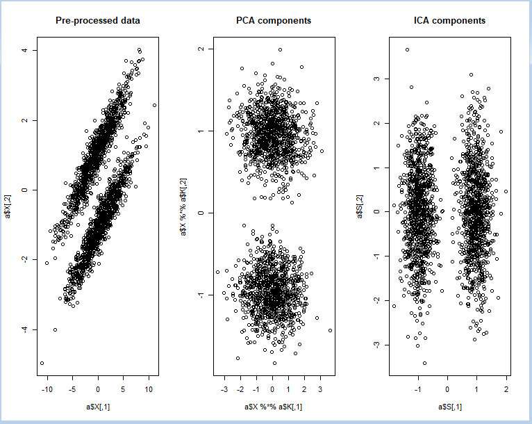
FastICA to perform projection pursuit on a mixture of bivariate normal distributions using R
#R Code 3: using FastICA to perform projection pursuit on a mixture of bivariate normal distributions

if(require(MASS)){
x <- mvrnorm(n = 1000, mu = c(0, 0), Sigma = matrix(c(10, 3, 3, 1), 2, 2))
x1 <- mvrnorm(n = 1000, mu = c(-1, 2), Sigma = matrix(c(10, 3, 3, 1), 2, 2))
X <- rbind(x, x1)
a <- fastICA(X, 2, alg.typ = "deflation", fun = "logcosh", alpha = 1,
method = "R", row.norm = FALSE, maxit = 200,
tol = 0.0001, verbose = TRUE)
par(mfrow = c(1, 3))
plot(a$X, main = "Pre-processed data")
plot(a$X %*% a$K, main = "PCA components")
plot(a$S, main = "ICA components")
}
Result of ICA in R
The above code containing the following components,
Result of ICA
The above code containing the following components,
Result of ICA
The above code containing the following components,
Components | |
X | Pre-processed data matrix. |
K | Pre-whitening matrix that projects data onto the first n.comp principal components. |
W | Estimated un-mixing matrix. |
A | Estimated mixing matrix. |
S | Estimated source matrix. |
Independent Component Analysis remains a powerful tool for data analysis and signal separatio. Its applications in biomedical engineering, finance, and telecommunications continue to expand. As computational power improves, ICA will likely play an even greater role in various scientific and industrial fields. By leveraging ICA, researchers and engineers can extract meaningful insights from complex datasets and improve decision-making processes.
You can also find some other data analysis content here.
Canonical Correlation Analysis (CCA)
Principle Component Analysis (PCA)