The Central Limit Theorem (CLT) is one of the most important concepts in statistics and probability theory. It explains why many real-world phenomena tend to approximate a normal distribution, even when the underlying data is not normally distributed. Understanding the CLT is crucial for anyone working with data, whether in science, business, or any field that involves statistical inference.
Introduction to Central Limit Theorem
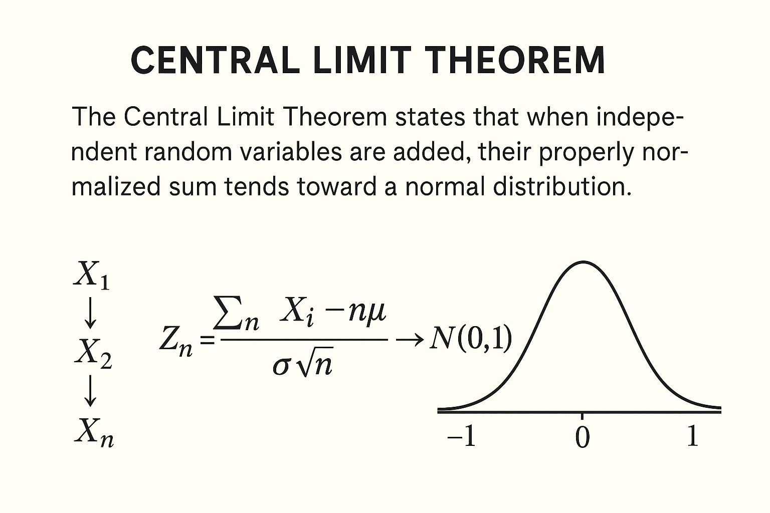
The Central Limit Theorem states that when independent random variables are added, their properly normalized sum tends toward a normal distribution (a bell curve), even if the original variables themselves are not normally distributed. This property allows statisticians to make inferences about population parameters from sample data.
Why is this important? Because the normal distribution is mathematically well-understood and has many useful properties. By knowing that the sum or average of a large enough sample behaves approximately normally, statisticians can apply numerous techniques such as hypothesis testing, confidence intervals, and regression analysis.
The Statement of the Central Limit Theorem
Suppose you have a sequence of independent and identically distributed (i.i.d.) random variables X1, X2,…,Xn each with mean μ and finite variance σ^2. Then the CLT says:

Here, Zn represents the standardized sum of random variables, and N(0,1) denotes the standard normal distribution with mean 0 and variance 1. The symbol →d stands for convergence in distribution.
In simpler terms, as the sample size n grows, the distribution of the sample sum (or average) approaches a normal distribution regardless of the original data’s distribution, provided the variance is finite.
Why the Central Limit Theorem Matters
- Prediction and Inference: The CLT allows us to use the normal distribution to approximate probabilities and critical values for sums or averages from various populations.
- Simplification: Even if the original data is skewed, has outliers, or is discrete, the CLT allows inference using the well-known normal curve.
- Foundation of Statistical Tests: Many inferential statistics methods, like t-tests and z-tests, rely on the CLT to justify their assumptions.
- Real-world applications: Finance, psychology, engineering, biology, and many other fields use CLT to analyze data and draw conclusions.
Understanding the Conditions of the Central Limit Theorem
The CLT holds under certain conditions:
- Independence: The random variables must be independent of one another.
- Identical distribution: Each random variable shares the same distribution.
- Finite variance: The variance σ2\sigma^2σ2 must be finite (not infinite or undefined).
When these conditions are satisfied, CLT applies well. However, there are generalizations of the CLT that relax some of these conditions.
Intuition Behind the Central Limit Theorem
Imagine you flip a biased coin many times. The number of heads follows a binomial distribution, which can be irregular for small trials. But if you flip it thousands of times, the distribution of the proportion of heads will resemble a smooth normal curve.
This occurs because the sum (or average) of many small independent random effects “smooth out” irregularities, resulting in a bell-shaped curve.
Examples Illustrating Central Limit Theorem
Example 1: Rolling Dice
A single dice roll produces a uniform distribution with values 1 through 6. If you roll a dice 1,000 times and calculate the average of the rolls, that average will approximately follow a normal distribution. The more rolls you take, the closer this distribution looks like a bell curve.
Example 2: Heights of People
The height distribution in a population might not be perfectly normal due to sampling or measurement errors, but the average height of random groups of people will approximate a normal distribution as group size increases.
Law of Large Numbers vs Central Limit Theorem
Both are fundamental in probability, but they differ:
| Aspect | Law of Large Numbers (LLN) | Central Limit Theorem (CLT) |
|---|---|---|
| Focus | Convergence of sample mean to population mean | Distribution of standardized sums or means |
| Nature | Deals with convergence almost surely | Deals with distributional convergence |
| Outcome | Sample mean becomes close to true mean | Distribution of sample mean tends to normal |
| Requires | Independence, identical distribution | Independence, identical distribution, finite variance |
Variations and Generalizations of the CLT
- Lindeberg-Levy CLT: The classical form for i.i.d. variables.
- Lindeberg-Feller CLT: Extends the theorem to independent but not identically distributed variables.
- Multivariate CLT: The sum of vectors of random variables converges to a multivariate normal distribution.
- Stable Distributions: CLT doesn’t hold if variance is infinite. Instead, sums may converge to other stable distributions such as Lévy distributions.
Practical Applications of Central Limit Theorem
- Quality Control: Monitoring products using sample averages assumes normality due to CLT.
- Polling: Pollsters use sample means to estimated population parameters, relying on CLT.
- Finance: Pricing models for returns of an asset often assume returns are normally distributed due to CLT.
- Machine Learning: Algorithms often assume data approximates normality, especially in large datasets.
How to Use the Central Limit Theorem in Statistical Analysis
- Collect sample data and compute the sum or average.
- Standardize the sample statistic by subtracting the mean and dividing by the standard error.
- Use the standard normal distribution to find probabilities or critical values.
- Make decisions or inferences based on these probabilities (e.g., confidence intervals, hypothesis testing).
Limitations of the Central Limit Theorem
- For small sample sizes, the approximation to a normal distribution may be poor.
- If data have infinite variance or very heavy tails, CLT may not apply.
- Data must be independent; correlated data violate assumptions.
- Not all sums converge to normal; some converge to other stable laws.
Conclusion
The Central Limit Theorem is a cornerstone of statistical theory and practice. It provides the justification for using normal distribution approximations when dealing with sums or averages of random variables, no matter their original distribution. This powerful theorem enables statisticians, scientists, and analysts to generalize results from samples to populations and apply a wide range of inferential techniques. Understanding the CLT’s assumptions, applications, and limitations is essential for properly interpreting data and making sound decisions in uncertain situations. Data Science Blog
Q&A on Central Limit Theorem
Q1: Why does the Central Limit Theorem work even if the original data is not normal?
A: The CLT works because the sum or average of many independent random variables tends to smooth out irregularities and extreme values, making the distribution of the standardized sums converge to a normal distribution regardless of the original shape.
Q2: How large should the sample size be for the CLT to hold?
A: There is no strict rule, but a sample size of 30 or more is often considered sufficient for many practical applications. The required size depends on the original distribution’s shape; more skewed or heavy-tailed data require larger samples.
Q3: Does the CLT apply to dependent data?
A: The classical CLT assumes independence. There are other versions of the theorem for dependent data, but these often require specific conditions such as weak dependence or mixing.
Q4: What happens if the variance is infinite?
A: If variance is infinite (e.g., heavy-tailed distributions like Cauchy), the CLT does not apply. In such cases, sums of random variables converge to different stable distributions, not the normal.
Q5: Can the CLT be used for medians or other statistics?
A: The classical CLT applies specifically to sums or averages. Other statistics, like medians, require separate asymptotic results and do not generally converge to a normal distribution in the same way.