In this session, we are going to learn how to manipulate, compute, and check the reliability of our variables. Variable manipulation and reliability check is an essential step of data analysis. In this article we will also learn how to re-code the response of our variables and compute to a new variable of our interest.
Re-coding Variable (variable manipulation and reliability check)
Why re-coding necessary?
We may need to re-code our variables for a variety of reasons. First and foremost, if our variable is abnormally skewed or not normally distributed, and we want to make the response to that variable less skewed so that our results are improved by using a proportionate response to our variable. Take a look at this variable—number of absences—in this dataset, for example (file name: studentdata2008). Students wrote down their total number of absences since the start of the current academic year in response to this variable. The number of times a response is given ranges from 0 through multiples of one. We would do the command tab to get the detail list of each response of “absent” variable. Here is how it looks like:
tab absentOnly a few students were absent more than six times, as shown in the table above. As a result, our results were weighted toward 0-5 times. The Skewness value of this variable is 2.49, and the Kurtosis value is 11.15, indicating that it is extremely skewed (see the short and sweet description of Skewness and Kurtosis here for more information). In this scenario, we’d recode the variable by merging those who were absent more than 6 times into a single group and labeling it “more than 6 times.” We don’t touch 0-5; leave them alone. To recode this variable, use this command: recode absent (0=0)(1=1)(2=2)(3=3)(4=4)(5=5)(6/25=6). Here is how it looks like:
Stata Code
recode absent (0=0)(1=1)(2=2)(3=3)(4=4)(5=5)(6/25=6)That is what we get based on that recode command above. Next, tab absent again, and we will see that the response 6-25 was combined. Here is how it looks like:
tab absent Now our variable absent looks like it’s normally distributed. The Skewness was reduced to 0.57 and Kurtosis to 1.88. The rule of thumb of a normally distributed variable would be a skewness of 1 and lower (nearer to zero is better) and Kurtosis of lower than 3.
So how did we get the values of Skewness and Kurtosis of the absent variable?
Type command summary (or sum) of absent variable by requesting detail (or simply d for shortcut). Here is how it looks like:
sum absent, detailSo there we have the values of Skewness and Kurtosis. The values indicate that our variable absent looks normally distributed. Below is a screenshot of how Skewness and Kurtosis are mentioned in a journal article.
Categorize Variable
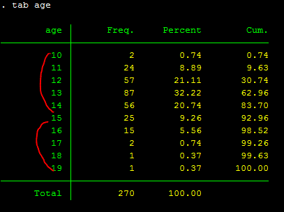
Another reason for recoding a variable is when we wish to categorize the response. Again, this is a very subjective exercise with a specific goal in mind. Consider the variable “age.” The respondents’ ages range from 10 to 19. If we want to divide them into five age categories, we’ll have two options: 10-14 and 15-19. The procedures would be the same as the ones listed above. Here is how it looks like when we tab age:
tab ageNow let’s do recoding of age:
recode age (10/14=1)(15/19=2)
or
recode age (min/14=1) (15/max=2)
I would recommend we to label this age variable as its values have been recoded so that we can still remember when we come back to the data in the future. Use the command: label var age “5-year range of age, 1=10-14 and 2=15-19”; description inside the quotation mark can be anything we want to call. It’s for we to remember what it is we recoded. Here is how it looks like after we label it:
label var age "5-year range of age, 1=10-14 and 2=15-19"
tab age
There is another way to label values (1 or 2 for the age above) and have it displayed in the output table like this one above. So instead of showing 1 and 2 and look at the label of the variable in the red circle, we can have it shown 10-14 or 15-19 instead. Here is how we do it:
Stata Code
label define age1 1 10_14yrs 2 15_19yrs
label values age age1
The “age1” can be anything we want to call it, and have need something for we to define the value label. Another important thing to remember is that please be careful about the “hyphenate” and “dash” as Stata is sensitive to the hyphenate one. Stata would treat it as “from this to that.” So if it is a label we want to remember on our own, use “dash”. For the example above, if we write “10-14yrs, then Stata would not be running, and it shows an error message saying that it’s “invalid syntax.”
GENERATING NEW VARIABLES
Before we recode, we should always save our old variables in case we need to return to them later. We never know what will happen. If we don’t make a new one, we won’t be able to recall it when we’ve recoded it. I recommend that we create a new variable that is equivalent to the one we wish to work with at all times. The variables absence and age, for instance, are a nice illustration. We want to keep these variables around and recode the ones we generate for current use. Generating a variable can be done easily with the command: generate or gen for short.
Now let’s look at the variables absent again and generate a new one of it. A new variable that we generated (or created) can be called anything we would like to (but no spacing). I myself prefer to use rc adding to the new variable being generated so that I know that it is recoded. So for the absent variable, the newly generated one would be called “absent_rc”. So here is how it looks like:
gen absent_rc = absent Labeling the new Variable
And again, we should label this variable so that we won’t forget what it is called when we come back later. I assume that by now we know how to label our variables. So show me how we would do it!. After we have done it, the new label will appear in the yellow highlight part above. Please note that when we generate a new variable that is equivalent to our old one, the new one must be placed first, right after “gen” command. Remember, we generate new variable to be equal to the old one, if that helps we memorize.
Now that we have generate our new absent variable, we can use that one to do the recoding. Simple!
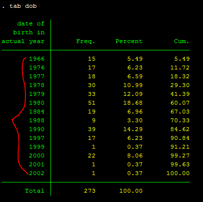
Command “gen” can be used to generate (or convert) values of our variables as well. For example, for our variable “dob” (date of birth in actual year), the response was in actual year. It looks like this by using tab command:
But we want to make this variable to actual age (let’s say in 2014, how old our participants are). First of we need to call this new variable that we want to generate into actual age. It is up to we what to call, but I would call it as “dob_age”. We can generate dob into year by using this one straight command: gen dob_age=(2014 – dob). [Note: it’s 2014 minus dob]:
gen dob_age=(2014 - dob) Now our dob variable has been converted into actual age, instead of year.
Let’s keep it simple for now about the use of gen command. There are many more functions that gen command can give we.
COMPUTE NEW VARIABLES (variable manipulation and reliability check)
When we have numerous variables that we want to average into a single variable, we can compute to a new variable. For example, there are eight variables in our Happiness Survey data that were utilized to quantify the participants’ physical issues. We generate a new single variable or scale that measures physical problem by combining or averaging the 8 factors together. We use command “gen” or “egen” to average these 8 variables: gen physical_problem = (Psleep + Pache + Phead + Peat + Ptired + Pfam + Pworry + Pfocus)/8. Here is how it looks like:
gen physical_problem = (Psleep + Pache + Phead + Peat + Ptired + Pfam + Pworry + Pfocus)/8Now we have created/computed/generated a new variable or a new measure for physical health. And again, we should label this variable so that we won’t forget what it is later. I assume that by now we know how to label our variable.
Another way to generate this physical problem variable, we can use “egen” command. It looks like this:
egen physical_problem = rmean (Psleep - Pfocus) That should also generate/compute our physical problem measure.
RELIABILITY CHECK
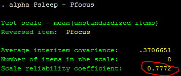
Before creating a measure like the one above, the physical problem one, it’s a good idea to see how reliable it is. To put it another way, how one item is related to the others. Inter-item dependability is the term for this. Cronbach’s alpha is a metric that we use to assess the consistency of a measure we’re trying to develop. A Cronbach’s alpha of 0.70 or above is considered good, while 0.80 or higher is considered highly dependable. Let’s have a look at how reliable the physical problem measure is. We can use the command: alpha. Here is how it looks like:
alpha Psleep - PfocusWhat it shows here is the alpha = 0.7772 (or .78). We can say that the physical problem measure is reliable. A value below .70 is usually not so welcomed by peer-reviewed journal.
This is an example of how this part of analysis is presented in a peer-reviewed journal.
So, this is all for variable manipulation and reliability check using stata.


