
The paired sample t-test, sometimes called the dependent sample t-test, is a statistical procedure used to determine whether the mean difference between two sets of observations is zero. In a paired sample t-test, each subject or entity is measured twice, resulting in pairs of observations. The steps involved in paired sample t-test are following:
- Introduction
- Formulation of hypothesis
- Example data set
- Descriptive analysis
- Association or correlation test
- Visualizing samples
- Homogeneity in variances
- Paired sample t-test
- Interpretation
Introduction
Paired sample T-test is also called the dependent sample T-test. It compares differences between two dependent mean scores. It is used to determine whether the mean difference between two sets of observations is zero. In a paired sample t-test each subject or entity is measured twice. This results in pairs of observations. The common application of paired sample t-test includes case-control studies or repeated measures.
The paired sample t-test has the following assumptions:
- The dependent variable must be numeric and continuous
- Observations are independent of one another
- The dependent variable should be approximately normally distributed
- Dependent variable should not contain any outliers
Let’s carry out paired sample t-test in R studio. Suppose you are interested in evaluating the effectiveness of a company training program. One approach you might consider would be to measure the performance of a sample of employees before and after completing the program and analyze the differences using a paired sample t-test.
Suppose a training program was conducted to improve the participants’ knowledge of ICT. Data were collected from a selected sample of 1010 individuals before and after the ICT training program. Test the hypothesis that the training is effective to improve the participants’ knowledge of ICT at 95% level of significance.
Formulation of hypothesis
Like many statistical procedures, the paired sample t-test has two competing hypotheses, the null hypothesis and the alternative hypothesis. The null hypothesis assumes that the true mean difference between the paired samples is zero. Under this model, all observable differences are explained by random variation. Conversely, the alternative hypothesis assumes that the true mean difference between the paired samples is not equal to zero.
- H0: there is no difference in participants’ knowledge before and after the ICT training
- H1: ICT training affected the participant’s knowledge
The alternative hypothesis can take one of several forms depending on the expected outcome. If the direction of the difference does not matter, a two-tailed hypothesis is used. Otherwise, an upper-tailed or lower-tailed hypothesis can be used to increase the power of the test.
Note: It is important to remember that hypotheses are never about data, they are about the processes which produce the data.Example data set
We shall test this hypothesis against the alternative hypothesis. The data is shown below:
ICT training data
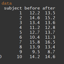
Let’s create this data set in Rstudio. First, create before and after as objects containing the scores of ICT training.
before <- c(12.2, 14.6, 13.4, 11.2, 12.7, 10.4, 15.8, 13.9, 9.5, 14.2)
after <- c(13.5, 15.2, 13.6, 12.8, 13.7, 11.3, 16.5, 13.4, 8.7, 14.6)
Now create a data matrix using data.frame() function. In this function, you can define the variables. The first variable is the subject or individuals. As the sample size is 1010 so we shall repeat 11 to 1010 twice. The second variable is time interval containing two levels. Each level will be repeated 1010 times. The third variable is ICT score representing response variable values. Use objects before and after as created earlier to represent scores. Let’s print the data to see how it looks like.
data <- data.frame(subject = rep(c(1:10), 2),
                   time = rep(c("before", "after"), each = 10),
                   score = c(before, after))
print(data)
# subject time score
# 1 1 before 12.2
# 2 2 before 14.6
# 3 3 before 13.4
# 4 4 before 11.2
# 5 5 before 12.7
# 6 6 before 10.4
# 7 7 before 15.8
# 8 8 before 13.9
# 9 9 before 9.5
# 10 10 before 14.2
# 11 1 after 13.5
# 12 2 after 15.2
# 13 3 after 13.6
# 14 4 after 12.8
# 15 5 after 13.7
# 16 6 after 11.3
# 17 7 after 16.5
# 18 8 after 13.4
# 19 9 after 8.7
# 20 10 after 14.6Use str() function to see the variable structure. The structure of the data variables is fine. The function attach() gives direct access to the variables of a data frame by typing the name of a variable as it is written on the first line of the file.
str(data)# 'data.frame': 20 obs. of 3 variables:
# $ subject: int 1 2 3 4 5 6 7 8 9 10 ...
# $ time : Factor w/ 2 levels "after","before": 2 2 2 2 2 2 2 2 2 2 ...
# $ score : num 12.2 14.6 13.4 11.2 12.7 10.4 15.8 13.9 9.5 14.2 ...attach(data)Descriptive analysis
Before proceeding for t-test let’s see the summary statistics of the data. Use summary() function to get the summary of scores. The summary() is a generic function used to produce result summaries of the results of various model fitting functions.
summary(data)# subject time score
# Min. : 1.0 after :10 Min. : 8.70
# 1st Qu.: 3.0 before:10 1st Qu.:11.97
# Median : 5.5 Median :13.45
# Mean : 5.5 Mean :13.06
# 3rd Qu.: 8.0 3rd Qu.:14.30
# Max. :10.0 Max. :16.50You can also get a summary of each time interval using by() function. In data argument type the name of the data file which was created as object earlier. In INDICES argument specify the second variable in quotation marks within square brackets. This will specify the time variable to split it into its components. Putting summary in FUN argument will apply summary to each component.
by(data = data,
   INDICES = data[,"time"],
   FUN = summary)
# data[, "time"]: after
# subject time score
# Min. : 1.00 after :10 Min. : 8.70
# 1st Qu.: 3.25 before: 0 1st Qu.:12.95
# Median : 5.50 Median :13.55
# Mean : 5.50 Mean :13.33
# 3rd Qu.: 7.75 3rd Qu.:14.38
# Max. :10.00 Max. :16.50
# ------------------------------------------------------------
# data[, "time"]: before
# subject time score
# Min. : 1.00 after : 0 Min. : 9.50
# 1st Qu.: 3.25 before:10 1st Qu.:11.45
# Median : 5.50 Median :13.05
# Mean : 5.50 Mean :12.79
# 3rd Qu.: 7.75 3rd Qu.:14.12
# Max. :10.00 Max. :15.80You may be interested in the summary statistics of the difference in scores before and after ICT training. Subtract the ICT score before training from the one after training to get the score differences. Again using the summary function for diff object will result in summary statistics for the differences.
diff = after - before
summary(diff)
# Min. 1st Qu. Median Mean 3rd Qu. Max.
# -0.800 0.250 0.650 0.540 0.975 1.600Association or correlation test
Now let’s see the association or correlation between the paired samples. Use cor.test() function to test this association. Type the components of the time variable in x and y arguments. In the method argument, we shall use Pearson which is the most commonly used method. Let’s test this relationship at 0.95 confidence level.
library(stats)
cor.test(x = before, y = after,
         method = c("pearson"),
         conf.level = 0.95)
#
# Pearson's product-moment correlation
#
# data: before and after
# t = 7.5468, df = 8, p-value = 6.628e-05
# alternative hypothesis: true correlation is not equal to 0
# 95 percent confidence interval:
# 0.7474506 0.9851801
# sample estimates:
# cor
# 0.9363955The results show that there is a significantly strong relationship between before and after training scores. The correlation coefficient is 0.940.94 which is very close to one. It reflects a strong positive relationship or association in before and after ICT training scores.
Visualizing samples
Its good practice to visualize the data set before applying test statistics. To set query of graphical parameters use par() function. To specify square plotting region of the plot set “s” for pty argument. To produce a box plot use boxplot() function where the argument formula is set to score ~ time. You can add additional arguments like col to set colors, main to add title and xlab and ylab arguments to add labels to X and Y-axis labels.
par(pty = "s")
boxplot(score ~ time)
boxplot(score ~ time,
        col = c("#003C67FF", "#EFC000FF"),
        main = "ICT training score improves knowlege",
        xlab = "Time", ylab = "Score")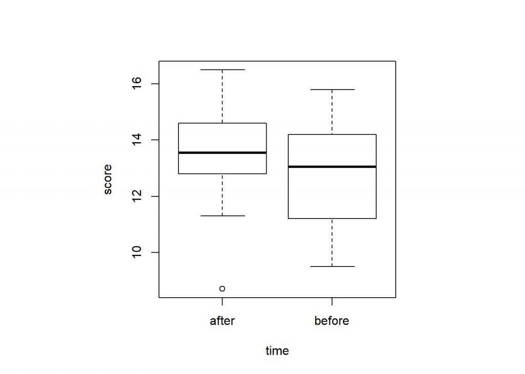

In a box plot we can get the information of distributional characteristics:
- Upper and lower whisker represents the scores outside the middle 50 percent
- Upper and lower quartiles
- 75 percent of the scores fall below the upper quartile and 25% of the scores fall below the lower quartile
- The middle box represents the middle 50 percent of the score (Interquartile range)
- The median or middle quartile represent the midpoint of the data
Characteristics of boxplot
Homogeneity in variances
Before proceeding with test statistics, first determine the homogeneity of variances of time variables for ICT training scores. You can use bartlett.test() where the score is separated by time variable.
bartlett.test(score ~ time)#
# Bartlett test of homogeneity of variances
#
# data: score by time
# Bartlett's K-squared = 0.050609, df = 1, p-value = 0.822The probability value is 0.820.82 which is higher than 0.050.05. This indicated that there is no significant difference in variances. It also means variances are homogeneous.
Paired sample t-test
Now let’s apply the paired sample t-test on data set by using t.test() function. Set the value for formula argument as score is separated by time. In alternative argument set the value of alternative hypothesis as “two.sided” in this case for two tailed hypothesis. The mu argument indicate the true value of difference in means for a two sample test. You can set the value of this argument according to the null hypothesis as in this case null hypothesis is the hypothesis of no difference (H0:μ1−μ2=0H0:μ1−μ2=0). Set TRUE for paired argument as this is paired sample data and each subject is measured twice before and after the ICT training. The variances are homogeneous as indicated by the test of homogeneity computed earlier so set TRUE for var.equal argument. Keep confidence level at 0.950.95 in conf.level argument. This corresponds to 9595 percent chance of obtaining a result like the one that was observed if the null hypothesis was false.
t.test(formula = score ~ time,
       alternative = "greater",
       mu = 0,
       paired = TRUE,
       var.equal = TRUE,
       conf.level = 0.95)
#
# Paired t-test
#
# data: score by time
# t = 2.272, df = 9, p-value = 0.0246
# alternative hypothesis: true difference in means is greater than 0
# 95 percent confidence interval:
# 0.1043169 Inf
# sample estimates:
# mean of the differences
# 0.54Interpretation
Statistical significance is determined by looking at the p-value. The p-value gives the probability of observing the test results under the null hypothesis. The lower the p-value, the lower the probability of obtaining a result like the one that was observed if the null hypothesis was true. Thus, a low p-value indicates decreased support for the null hypothesis.
The results showed that the probability value is lower than 0.05. Lower the P-value, lower the evidence we have to support the null hypothesis. Based on this result, we shall reject the null hypothesis of no difference. It means ICT training significantly improved the participants’ knowledge.