
A general linear model (GLM) with at least one continuous and one categorical independent variable is known as ANCOVA (treatments). When the effect of treatments is essential and there is an additional continuous variable in the study, ANCOVA is effective. A covariate is an additional continuous independent variable in ANCOVA (also known as a control, concomitant, or confounding variable). By statistically modifying the influence of the covariate, ANCOVA evaluates the differences between groups in a categorical independent variable (primary interest) (by removing the variance associated with the covariate).
By reducing the variance associated with a covariate, ANCOVA improves statistical power and decreases error terms. ANCOVA calculates adjusted means for each group in a categorical independent variable (which are statistically controlled for covariates). Adjusted means eliminating the model’s covariate bias. ANCOVA examines the adjusted effects of the independent variable on the dependent variable using a multiple regression method (similar to simple regression in ANOVA).
ANCOVA example
The following hypothetical example data consists of two independent variables viz. plant genotype (categorical) and plant genotype height (continuous). The yield ofthe plant genotype is the dependent variable. The ANCOVA model analyzes the influence of plant genotypes on genotype yield whilst controlling the effect of the covariate. With ANCOVA, the effect of different genotypes on plant yield can be precisely analyzed while controlling for the effect of plant height.
Assumptions of ANCOVA
ANCOVA follows similar assumptions as in ANOVA for the independence of observations, normality, and homogeneity of variances
In addition, ANCOVA needs to meet the following assumptions,
- Linearity assumption: At each level of the categorical independent variable, the covariate should be linearly related to the dependent variable. If the relationship is not linear, the adjustment made to the covariate will be biased.
- Homogeneity of within-group regression slopes (parallelism or non-interaction): There should be no interaction between the categorical independent variable and covariate i.e. the regression lines between the covariate and dependent variable for each group of the independent variable should be parallel (same slope).
- Dependent variable and covariate should be measured on a continuous scale
- Covariate should be measured without error or as little error as possible
One-way (one factor) ANCOVA in R
In one-way ANCOVA, there are three variables, viz. one independent variable with two or more groups, dependent, and covariate variables
ANCOVA Hypotheses
- Null hypothesis: Means of all genotypes yield are equal after controlling for the effect of genotype height i.e., adjusted means are equal
H0: μ1=μ2=…=μp - Alternative hypothesis: At least one genotype yield mean is different from the other genotypes after controlling for the effect of genotype height i.e., adjusted means are not equal
H1: All μ’s are not equal
Load the dataset
library(tidyverse)
df=read_csv("https://reneshbedre.github.io/assets/posts/ancova/ancova_data.csv")
head(df, 2)
# output
  genotype height yield
  <chr>     <dbl> <dbl>
1 A          10      20
2 A          11.5    22
Summary statistics and visualization of the dataset
Get summary statistics based on the dependent variable and covariate,
library(rstatix)
# summary statistics for dependent variable yield
df %>% group_by(genotype) %>%  get_summary_stats(yield, type="common")
# output
  genotype variable     n   min   max median   iqr  mean    sd    se    ci
  <chr>    <chr>    <dbl> <dbl> <dbl>  <dbl> <dbl> <dbl> <dbl> <dbl> <dbl>
1 A        yield       10    20  27.5   26.5  3     25.2  2.58 0.815  1.84
2 B        yield       10    32  40     36    3.62  35.4  2.43 0.769  1.74
3 C        yield       10    15  21     17.7  2.88  17.7  2.04 0.645  1.46

# summary statistics for covariate height
df %>% group_by(genotype) %>%  get_summary_stats(height, type="common")
# output
 genotype variable     n   min   max median   iqr  mean    sd    se    ci
  <chr>    <chr>    <dbl> <dbl> <dbl>  <dbl> <dbl> <dbl> <dbl> <dbl> <dbl>
1 A        height      10    10  16.6   13.8  3.45  13.8  2.22 0.704  1.59
2 B        height      10    14  20     16.5  2.6   16.8  1.96 0.621  1.40
3 C        height      10     7  12      9.9  2.55   9.6  1.84 0.582  1.32
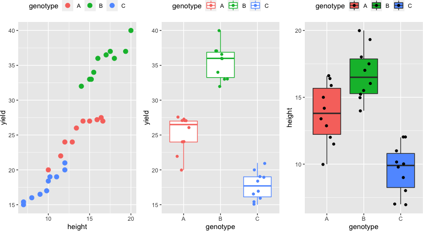
Visualize the dataset,
library(gridExtra)
p1 <- ggplot(df, aes(height, yield, colour = genotype)) + geom_point(size = 3) + theme(legend.position="top")
p2 <- ggplot(df, aes(x = genotype, y = yield, col = genotype)) + geom_boxplot(outlier.shape = NA) + geom_jitter(width = 0.2) + theme(legend.position="top")
p3 <- ggplot(df, aes(x = genotype, y = height, fill = genotype)) + geom_boxplot(outlier.shape = NA) + geom_jitter(width = 0.2) + theme(legend.position="top")
grid.arrange(p1, p2, p3, ncol=3)
Perform one-way ANCOVA
anova_test(data = df, formula = yield ~ height + genotype, type = 3, detailed = TRUE) # type 3 SS should be used in ANCOVA
# output
ANOVA Table (type III tests)

       Effect     SSn    SSd DFn DFd       F        p p<.05   ges
1 (Intercept)  78.071 17.771   1  26 114.220 5.22e-11     * 0.815
2      height 132.696 17.771   1  26 194.138 1.43e-13     * 0.882
3    genotype 193.232 17.771   2  26 141.353 1.07e-14     * 0.916
ANCOVA results indicate that there are significant differences in mean yield [F(2, 26) = 141.35, p < 0.001] among genotypes whilst adjusting for the effect of genotype height.
The covariate height is significant [F(1, 26) = 194.13, p < 0.001], suggesting it is an important predictor of genotype yield.
Get adjusted means,
adj_means <- emmeans_test(data = df, formula = yield ~ genotype, covariate = height)
get_emmeans(adj_means)
# output
 height genotype emmean    se    df conf.low conf.high method
   <dbl> <fct>     <dbl> <dbl> <dbl>    <dbl>     <dbl> <chr>
1   13.4 A          24.7 0.263    26     24.2      25.3 Emmeans test
2   13.4 B          31.7 0.373    26     31.0      32.5 Emmeans test
3   13.4 C          21.9 0.397    26     21.1      22.7 Emmeans test
emmeans gives the estimated marginal means (EMMs) which is also known as least-squares means. EMMs are adjusted means for each genotype. The B genotype has the highest yield (31.7) whilst controlling for the effect of height.
Post-hoc Test
From ANCOVA, we know that genotypes yield are statistically significant whilst controlling for the effect of height, but ANCOVA does not tell which genotypes are significantly different from each other.
To know the genotypes with statistically significant differences, I will perform the post-hoc test with the Benjamini-Hochberg FDR method for multiple hypothesis testing at a 5% cut-off
emmeans_test(data = df, formula = yield ~ genotype, covariate = height, p.adjust.method = "fdr")
# output
  term  .y.   group1 group2    df statistic        p    p.adj
* <chr> <chr> <chr>  <chr>  <dbl>     <dbl>    <dbl>    <dbl>
1 heig… yield A      B         26    -16.0  5.32e-15 1.60e-14
2 heig… yield A      C         26      5.71 5.21e- 6 5.21e- 6
3 heig… yield B      C         26     14.6  4.89e-14 7.33e-14
The multiple pairwise comparisons suggest that there are statistically significant differences in adjusted yield means among all genotypes.
ANCOVA assumptions test
Assumptions of normality
The residuals should approximately follow a normal distribution. We can use the Shapiro-Wilk test to check the normal distribution of residuals. The null hypothesis states that the data comes from a normal distribution.
shapiro.test(resid(aov(yield ~ genotype + height, data = df)))
# output
	Shapiro-Wilk normality test

data:  resid(aov(yield ~ genotype + height, data = df))
W = 0.96116, p-value = 0.3315
Since the p-value is non-significant (p > 0.05), we fail to reject the null hypothesis and conclude that the data comes from a normal distribution.
If the sample size is sufficiently large (n > 30), the moderate departure from normality can be allowed.
In addition, we can use QQ plots and histograms to assess the assumptions of normality.
Assumptions of homogeneity of variances
The variance should be similar for all genotypes. We can use Bartlett’s test to check the homogeneity of variances. Null hypothesis: Samples from populations have equal variances.
bartlett.test(yield ~ genotype, data = df)
# output
	Bartlett test of homogeneity of variances

data:  yield by genotype
Bartlett's K-squared = 0.48952, df = 2, p-value = 0.7829
As the p-value is non-significant (p > 0.05), we fail to reject the null hypothesis and conclude that genotypes have equal variances.
Levene’s test can be used to check the homogeneity of variances when the data is not drawn from a normal distribution.
Assumptions of homogeneity of regression slopes (covariate coefficients)
This is an important assumption in ANCOVA. There should be no interaction between the categorical independent variable and the covariate. This can be tested using interaction terms between genotype and height in ANOVA. If this assumption is violated, the treatment effect won’t be the same across various levels of the covariate. At this stage, consider alternatives to ANCOVA, such as Johnson Neyman Technique.
Anova(aov(yield ~ genotype * height, data = df), type = 3)
# output
                Sum Sq Df F value    Pr(>F)
(Intercept)     24.140  1 32.8418 6.629e-06 ***
genotype         6.756  2  4.5960   0.02042 *
height          52.014  1 70.7635 1.283e-08 ***
genotype:height  0.130  2  0.0887   0.91545
Residuals       17.641 24
As the p-value for interaction (genotype: height) is non-significant (p > 0.05), there is no interaction between genotype and height.
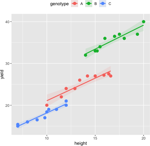
Assumptions of linearity
The relationship between the covariate and each group of the independent variable should be linear. We can use the scatterplot of the covariate and dependent variable at each group of the independent variable to assess this assumption. The data points should lie on a straight line to meet the linearity assumption.
ggplot(df, aes(height, yield, colour = genotype)) + geom_point(size = 3) +
    geom_smooth(method = "lm", aes(fill = genotype), alpha = 0.1) + theme(legend.position="top")
Interpreting ANCOVA Results
When interpreting ANCOVA output, you typically look at:
- Significance of the Covariate: First, check if the covariate is significantly related to the dependent variable. A significant p-value for the covariate indicates that it explains a meaningful portion of the variance in the dependent variable, justifying its inclusion in the model.
- Homogeneity of Regression Slopes Test: As discussed, this is critical. If the interaction term between the IV and CV is non-significant, you can proceed with interpreting the main effects. If significant, the interpretation changes, and you cannot simply interpret the main effect of the independent variable without considering the covariate’s differential effect.
- Main Effect of the Independent Variable (Adjusted for Covariate): If the homogeneity of slopes assumption is met, we then examine the F-statistic and p-value for the independent variable. A significant p-value here indicates that there are statistically significant differences in the adjusted means of the dependent variable across the levels of your independent variable, after controlling for the covariate.
- Estimated Marginal Means (EMMs): These adjusted group means provide a clear picture of the group differences after the analysis statistically removes the covariate’s influence. Researchers often present them in tables or plots.
- Effect Size (e.g., Partial Eta Squared): This metric indicates the proportion of variance in the dependent variable explained by the independent variable after accounting for the covariate. It helps in assessing the practical significance of the findings.
ANCOVA vs. ANOVA vs. Regression
It’s helpful to understand how ANCOVA relates to its statistical cousins:
- ANOVA (Analysis of Variance): Used to compare the means of two or more groups on a continuous dependent variable. It’s suitable when you only have categorical independent variables and no continuous confounding variables to control for.
- Regression Analysis: Used to model the relationship between a continuous dependent variable and one or more independent variables (which can be continuous or categorical, often using dummy coding for categorical variables). Regression focuses on predicting the dependent variable based on the independent variables.
- ANCOVA: Essentially a blend of ANOVA and regression. It allows you to compare group means (like ANOVA) while simultaneously accounting for the linear effect of continuous covariates (like regression).
In a sense, you can perform ANCOVA using multiple regression by including dummy variables for the categorical independent variable and the continuous covariate(s).
| Feature | ANOVA | Regression | ANCOVA |
|---|---|---|---|
| Primary Goal | Compare group means | Predict a dependent variable | Compare group means, controlling for continuous covariates |
| Independent Var. | Categorical | Continuous and/or Categorical | Categorical (factors) and Continuous (covariates) |
| Dependent Var. | Continuous | Continuous | Continuous |
| Controlling for | Not designed for continuous confounders | Controls for all included predictors | Specifically controls for continuous covariates, increasing precision |
| Underlying Math | Variance decomposition | Least squares minimization | Combines variance decomposition and least squares minimization |
Conclusion
ANCOVA is a powerful and versatile statistical technique that significantly enhances the precision and validity of research findings, particularly in studies where confounding continuous variables are present. By integrating the strengths of both ANOVA and regression, ANCOVA enables researchers to draw more accurate conclusions about the true effects of their independent variables, leading to a deeper and more nuanced understanding of complex phenomena. However, a thorough understanding of its assumptions and careful interpretation of its results are paramount for its effective and ethical application. Data Science Blog